10.4 Interactions: letting the slope differ
A dummy shifts the line up or down. What if the groups differ in more than that?
Everything so far has moved the intercept. The model
\[\ln(\text{earnings}) = \beta_0 + \beta_1\,\text{educ} + \beta_2\,\text{urban} + u\]
fits two lines, one for each group, but forces them to be parallel. Urban workers earn more at every level of education, by the same amount.
That is an assumption, and there is no reason to believe it. The return to a year of schooling might itself differ between rural and urban labour markets.
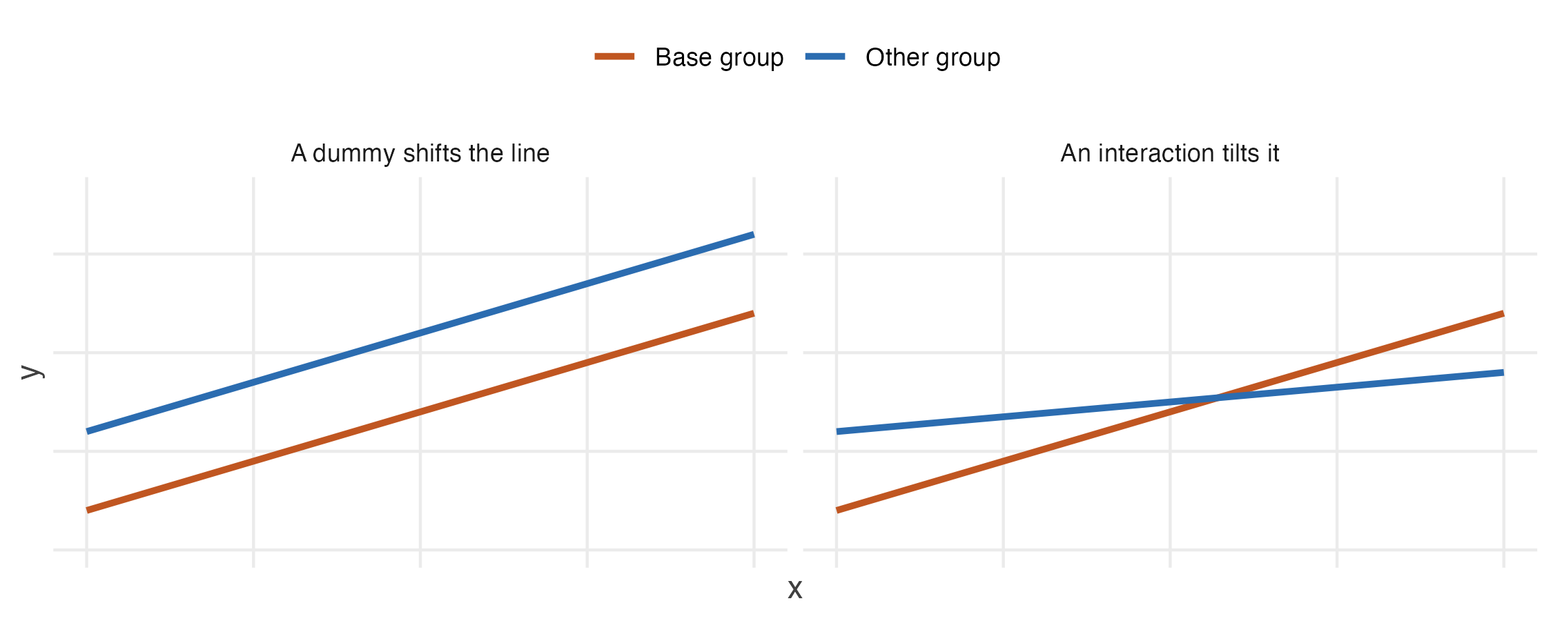
Figure 10.1: The two things a group variable can do. On the left the groups differ only in level, which is all a dummy on its own can express. On the right they differ in level and in rate of change, which requires an interaction term.
A dummy variable shifts. An interaction tilts.
To allow the tilt, add the product of the two variables.
\[\ln(\text{earnings}) = \beta_0 + \beta_1\,\text{educ} + \beta_2\,\text{urban} + \beta_3\,(\text{educ} \times \text{urban}) + u\]
The product is called an interaction term.
Substitute the two possible values of the dummy, as before.
For rural workers, \(\text{urban} = 0\), so both terms containing it vanish:
\[E[\ln(\text{earnings})] = \beta_0 + \beta_1\,\text{educ}\]
For urban workers, \(\text{urban} = 1\):
\[ \begin{aligned} E[\ln(\text{earnings})] &= \beta_0 + \beta_1\,\text{educ} + \beta_2 + \beta_3\,\text{educ} \\[4pt] &= (\beta_0 + \beta_2) + (\beta_1 + \beta_3)\,\text{educ} \end{aligned} \]
So the model fits two completely separate lines:
- \(\beta_2\) is the difference in intercepts;
- \(\beta_3\) is the difference in slopes.
#>                 Estimate Std. Error t value Pr(>|t|)
#> (Intercept)      9.41615    0.01332  706.96  0.00000
#> education        0.07977    0.00192   41.47  0.00000
#> urban            0.95865    0.03012   31.83  0.00000
#> education:urban -0.01090    0.00354   -3.08  0.00208
R expands education * urban into education + urban + education:urban.
Read the four numbers as two lines:
b <- coef(interacted)

round(rbind(rural = c(intercept = b[1],           slope = b[2]),
            urban = c(intercept = b[1] + b[3],    slope = b[2] + b[4])), 5)
#> intercept.(Intercept) slope.education
#> rural 9.416 0.07977
#> urban 10.375 0.06886For rural workers a year of schooling is worth about 8.0%; for urban workers, about 6.9%. The interaction coefficient is \(-0.0109\) with a \(t\) statistic of \(-3.08\), so the difference is more than sampling variation would produce.
With an interaction in the model, \(\beta_1\) is not “the effect of education”.
It is the effect of education in the base group only — here, rural workers. The urban return requires adding the interaction coefficient.
This is the same warning as the squared term of Section 9.6, and for the same reason: once a variable appears twice, no single coefficient answers the question on its own.
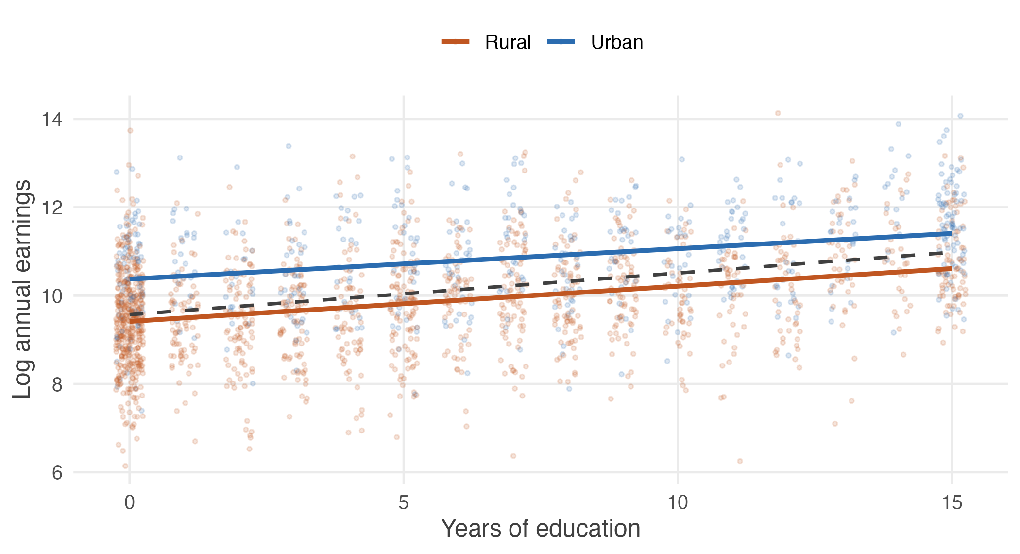
Figure 10.2: Log earnings against education for rural and urban workers, with a 2,000-worker sample drawn for legibility. The solid lines are fitted separately to each group; the dashed line is the single pooled regression that ignores residence. The two group lines differ in level and, less obviously, in steepness – the urban line is slightly flatter. The pooled line describes neither group.
An interaction is how a regression says “it depends”.
Without one, the model insists that education is worth the same everywhere and that living in a city is worth the same at every level of schooling. With one, each answer is allowed to depend on the other.
Note that the dependence runs both ways, and reading it either way is legitimate. The return to education differs by residence; equivalently, the urban premium differs by education. The same coefficient says both, because \(\text{educ} \times \text{urban}\) does not know which variable we regard as primary.