1.4 What if we repeated the survey?

If our conclusions depend on the particular sample we happened to observe, how can we learn anything about the population?

The previous section ended with a simple but unsettling observation. A different sample produces a different mean. The same is true of the median, the standard deviation and every other statistic we compute.

One possibility is to collect another sample.

Imagine repeating the survey. A new team visits a different set of households, following exactly the same sampling design. They compute the average annual earnings and obtain a value that differs slightly from the first survey.

Now imagine repeating the exercise again.

And again.

Every new survey produces a new sample, and every sample produces a new mean. None of these means is “correct” or “incorrect”. Each is simply the result of observing a different subset of the population.

Of course, conducting thousands of nationwide surveys would be prohibitively expensive. Fortunately, we do not need to. Since we are treating our dataset as the population for the purposes of this chapter, we can recreate this thought experiment on a computer.

Suppose we repeatedly draw random samples of 2,000 workers from our population. For each sample we calculate the mean annual earnings and store the result. After repeating this process one thousand times, we have one thousand sample means.

set.seed(1)

sample_means <- replicate(
  1000,
  mean(sample(workers$annual_earnings,
              size = 2000,
              replace = TRUE))
)

What do these one thousand means look like?

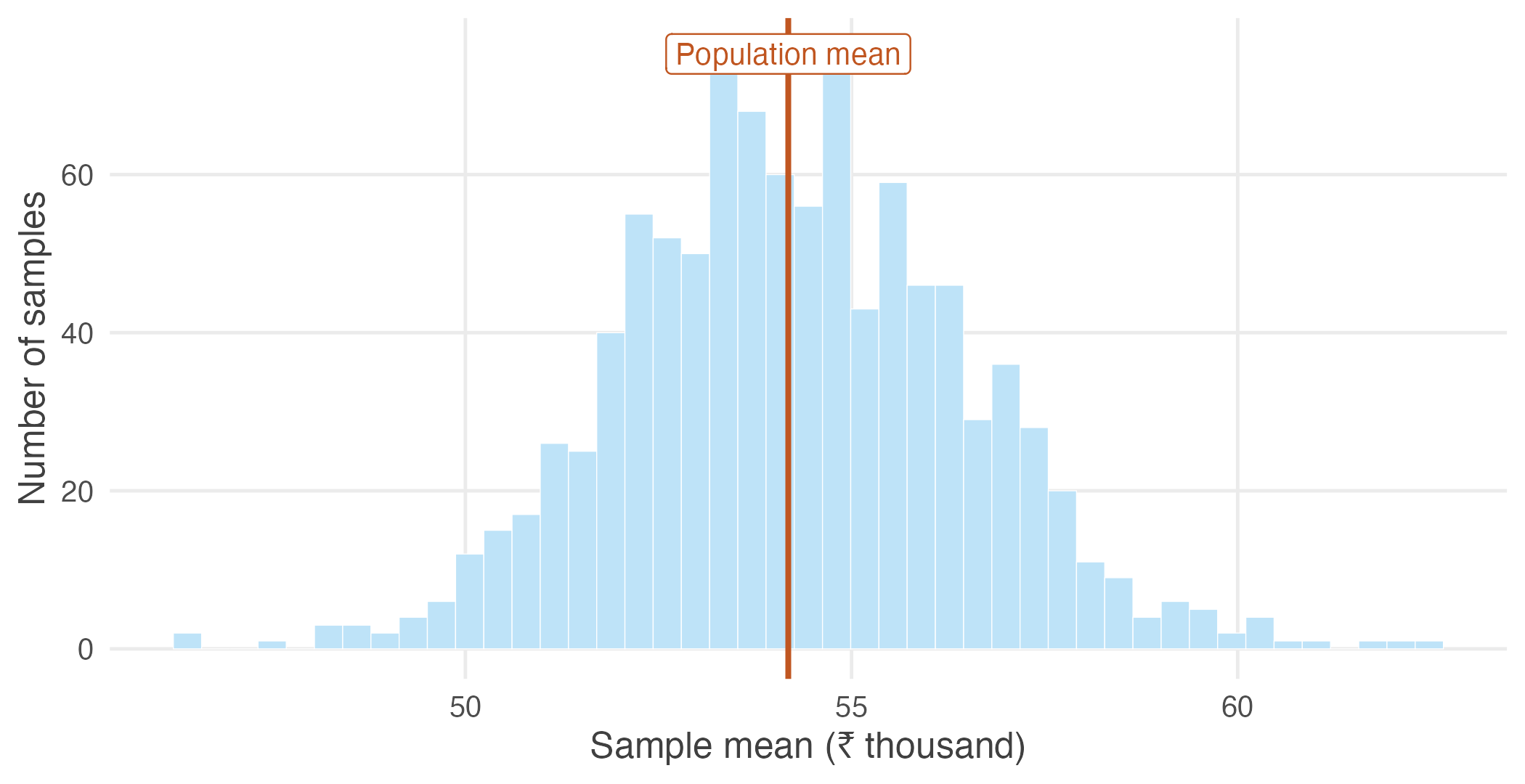
Figure 1.5: Distribution of the sample mean based on 1,000 samples of 2,000 workers.

Several features stand out immediately.

First, the sample means are not all identical. Even though every sample was drawn from the same population using the same procedure, each survey produced a slightly different average.

Second, the variation is not arbitrary. Most of the sample means cluster within a relatively narrow range, while only a few lie far from the centre. Extreme values are possible, but they are uncommon.

Finally, the distribution itself has a remarkably regular shape. Although the earnings of individual workers are highly skewed, the distribution of the sample means is much more symmetric and concentrated.

The thousand means are not just a collection of numbers. They form a distribution of their own. Notice what this distribution describes. It is not the distribution of workers’ earnings — that was the distribution we began with. Instead, it is the distribution of the sample mean obtained by repeating the survey many times. The object of interest has changed. We are no longer studying individual workers; we are studying the behaviour of the sample mean.

This distinction lies at the heart of inferential statistics. The original distribution describes the variability in earnings across workers. The new distribution describes the variability in the sample mean across repeated samples. It is this second source of variation that determines how much confidence we should place in the average computed from a single survey.

The distribution formed by a statistic over repeated samples is called its sampling distribution. Every statistic has a sampling distribution: the mean, the median, the standard deviation, and many others. In this chapter we focus on the sampling distribution of the sample mean because it provides the foundation for much of statistical inference.

Two features of Figure 1.5 are too striking to ignore. First, the sample means are tightly concentrated around the population mean. Second, despite the strong skewness of individual earnings, their sampling distribution is almost bell-shaped. Neither feature is a coincidence. Both are consequences of two fundamental results in probability theory: the Law of Large Numbers and the Central Limit Theorem. Together, these results explain why a single sample can provide reliable information about an entire population.