7.5 How precise is OLS?

The histogram had a width as well as a centre. Can we know that width from one sample?

The sampling distribution in Section 7.3 had a standard deviation of 0.0526. That number is exactly what we want: it says how far a slope from a single sample of forty is liable to fall from the truth.

But look at how we obtained it. We drew five thousand samples.

Nobody does that. A survey is run once, at considerable expense, and yields one sample and one slope. The standard deviation of the distribution those samples came from is not something we can watch.

So the question is this. Can we recover, from a single sample, the spread of a distribution we could otherwise see only by drawing thousands?

Remarkably, yes.

The formula

The width of the sampling distribution turns out to depend on two things, and both are things we can measure.

\[\mathrm{Var}(\hat{\beta}_1) = \frac{\sigma^2}{\sum(x_i - \bar{x})^2}\]

The numerator is the noise: how far individual observations scatter around the line. Noisier relationships are harder to pin down.

The denominator is the total variation in \(x\) — the same sum of squares we met in Section 7.2, computed on the explanatory variable rather than the outcome. It measures how much the data actually tell us about \(x\).

Since \(\sigma^2\) is unknown, it is estimated from the residuals. Two parameters were estimated on the way, so the divisor is \(n-2\) — the same accounting as Section 3.2, where estimating one mean cost one degree of freedom:

\[\hat{\sigma}^2 = \frac{\sum \hat{u}_i^2}{n - 2} \qquad\qquad \mathrm{se}(\hat{\beta}_1) = \frac{\hat{\sigma}}{\sqrt{\sum(x_i - \bar{x})^2}}\]

n <- length(y)
sigma_hat <- sqrt(sum(u_hat^2) / (n - 2))
se_b1     <- sigma_hat / sqrt(sum((x - mean(x))^2))

c(sigma_hat = sigma_hat, se_b1 = se_b1,
  se_from_lm = summary(fit)$coefficients[2, 2])

#>  sigma_hat      se_b1 se_from_lm 
#>    1.52697    0.01074    0.01074

Does it work?

A formula claiming to reconstruct a distribution we never observe deserves to be checked rather than believed.

Build a population where the assumptions hold exactly — a genuinely linear relationship, errors of constant variance — then draw from it repeatedly and compare what the formula says against what the samples actually do.

set.seed(4)
x_fixed <- runif(40, 2, 32)                    # forty students, attendance 2 to 32

check <- replicate(5000, {
  y_sim <- 1.56 + 0.189 * x_fixed + rnorm(40, sd = 1.53)
  m <- lm(y_sim ~ x_fixed)
  c(slope = coef(m)[2], se = summary(m)$coefficients[2, 2])
})

round(c(simulated_sd    = sd(check["slope.x_fixed", ]),
        average_formula = mean(check["se", ]),
        exact_formula   = 1.53 / sqrt(sum((x_fixed - mean(x_fixed))^2))), 4)

#>    simulated_sd average_formula   exact_formula 
#>          0.0287          0.0286          0.0287

The three agree to three decimal places. The formula, computed from one sample of forty, recovers the spread that five thousand samples reveal.

In other words: the standard error printed by lm() is an estimate of the standard deviation of the sampling distribution we simulated in Section 7.3.

That sentence connects the whole unit. The histogram is the thing; the standard error is our estimate of how wide it is, computed without ever drawing it.

Notice the words where the assumptions hold exactly. They were doing work.

Repeat the comparison on the real attendance data and the agreement is good rather than perfect: the formula gives about 0.046 for a sample of forty, while resampling gives about 0.053.

The formula is not wrong. Its assumptions are only approximately true here — Section 6.2 already showed the conditional mean of GPA is not exactly linear — and a formula inherits whatever inexactness its assumptions carry.

Which assumption is chiefly responsible in this particular dataset is not obvious and we shall not pretend otherwise. The general point stands regardless, and is worth holding on to whenever software prints a standard error to four decimal places: the number is only as good as the model behind it.

Why the denominator matters

Most readers remember that larger samples give smaller standard errors. Far fewer remember the other half, which is at least as important.

Look at the denominator again and ask what happens in extreme cases.

What if every student attended exactly 25 classes? Then \(x_i = \bar{x}\) for everyone, \(\sum(x_i - \bar{x})^2 = 0\), and the variance is undefined. There is no slope to estimate — we have observed grades at one attendance level and nothing about any other. This is assumption CLRM3, arriving as a consequence rather than a stipulation.

What if attendance varies only between 24 and 26? The denominator is small and the standard error is large. We are trying to infer a rate of change from almost no change.

What if attendance ranges from 2 to 32? The denominator is large and the slope is pinned down tightly.

The following figure makes the point with two datasets built from the same true line and the same error variance. Only the spread of \(x\) differs.

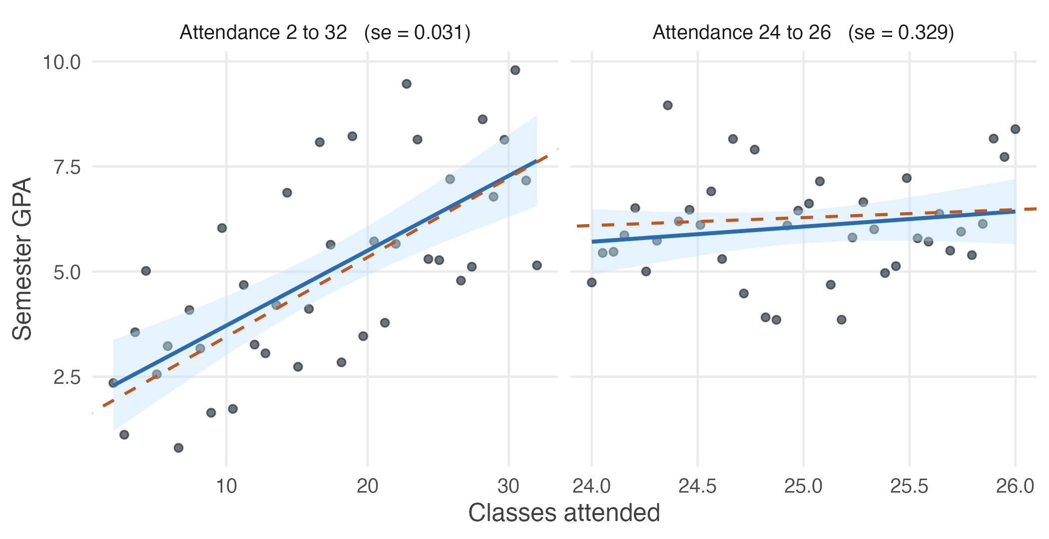
Figure 7.5: Two samples of forty from the same model: the same true slope of 0.189, the same noise, and the same sample size. Only the range of attendance differs. On the left the line is pinned down; on the right, where attendance varies by two classes rather than thirty, the same data are consistent with wildly different slopes.

The dashed orange line is the truth in both panels, and it is the same line.

On the left the fitted line sits almost on top of it: an estimated slope of 0.178 against a true 0.189. On the right the fitted slope is 0.360 — nearly twice the truth — and the shaded band around it is so wide as to be useless.

Note that the two panels have different horizontal scales, so compare the fitted lines to the dashed one within each panel rather than by eye across them.

Nothing about the relationship changed. Only the range over which we observed it.

A slope is a rate of change, and rates of change are measured by observing change.

Comparing students who attended 24 classes with students who attended 26 tells you very little about how attendance matters. Comparing those who attended 5 with those who attended 30 tells you a great deal.

Spread in the explanatory variable is information. A study that observes \(x\) over a narrow range will estimate its effect poorly however many observations it collects — which is also why the median split of Section 6.1 did so badly.

Where the formula comes from

Having seen that the formula works and what its parts mean, we can derive it.

One further assumption is needed, and it is worth seeing why. The derivation adds up the contributions of the individual errors, and to add them we must know how variable each one is. So far we have said nothing about that at all.

CLRM5 — homoskedasticity. \(\mathrm{Var}(u \mid x) = \sigma^2\), the same at every value of \(x\).

This is what allows a single number \(\sigma^2\) to stand in for the variability of every error. It played no part in unbiasedness, and Section 7.6 examines what happens when it fails.

Start from the expression that gave unbiasedness, and treat the \(x\)’s as fixed:

\[ \begin{aligned} \mathrm{Var}(\hat{\beta}_1) &= \mathrm{Var}\!\left(\beta_1 + \frac{\sum(x_i - \bar{x})u_i}{\text{SST}_x}\right) \\[4pt] &= \mathrm{Var}\!\left(\frac{\sum(x_i - \bar{x})u_i}{\text{SST}_x}\right) && \beta_1 \text{ is a constant} \\[4pt] &= \frac{1}{\text{SST}_x^2}\sum(x_i - \bar{x})^2\,\mathrm{Var}(u_i) && \text{independence} \\[4pt] &= \frac{\sigma^2 \,\text{SST}_x}{\text{SST}_x^2} && \text{homoskedasticity, CLRM5} \\[4pt] &= \frac{\sigma^2}{\text{SST}_x} \end{aligned} \]

Why is the slope estimated more precisely?

The standard error becomes smaller when

• the relationship is less noisy — small \(\sigma\);
• the sample is larger — more terms in \(\sum(x_i - \bar{x})^2\);
• the explanatory variable varies over a wider range — bigger terms in that same sum.

The last two both enter through the denominator, which is why \(n\) and the spread of \(x\) are not really two separate considerations. What matters is the total variation in \(x\), and either more observations or a wider range will increase it.

Those are the three findings of Section 7.3, now derived rather than observed. The second question mark in Table 7.1 is filled in.