4.1 The problem, before any formulas

The APU administration claims the average height of all students is 165 cm.

You are sceptical. You could settle it by measuring all 3,500 students, but that costs weeks of work. So instead you measure 36 students chosen at random, and you find their average height is 168 cm.

The claim said 165. Your sample says 168. Is the administration wrong?

The tempting answer is “yes, obviously — 168 is not 165.” That answer is wrong, and understanding why it is wrong is the whole chapter.

You did not measure everyone. You measured 36 people. Even if the true average really were exactly 165, your particular 36 students would almost never average exactly 165. Some samples come out high, some low. A gap between the sample and the claim is guaranteed to exist even when the claim is perfectly true.

Let us actually watch that happen.

We obviously do not know whether the administration is correct. But imagine, just for a moment, that they are. If the true average really were 165 cm, with a standard deviation of 8 cm, what kinds of sample means would we expect to see? Draw a sample of 36 students, ten separate times, and look.

set.seed(42)

ten_samples <- replicate(10, mean(rnorm(n = 36, mean = 165, sd = 8)))
round(ten_samples, 2)

#>  [1] 165.5 165.1 165.6 163.0 164.8 164.4 165.3 165.4 164.1 164.5

Every one of those numbers came from a population whose mean is exactly 165. Not one of them is 165. Several are further from 165 than a full centimetre.

So the real question is not “is 168 different from 165?” It obviously is. The real question is:

If the administration’s claim were true, how often would a sample of 36 students come out as far from 165 as ours did?

If the answer is “quite often” — then our sample is unremarkable, and we have no grounds to call anyone a liar.

If the answer is “almost never” — then either something very unusual happened to us, or the administration’s claim is not correct. In statistics we usually regard the second explanation as the more convincing one.

We can answer that question by brute force before we do any algebra at all. Let’s draw not ten samples but fifty thousand, still assuming the claim is true, and count how many stray at least 3 cm away from 165 (as ours did).

set.seed(42)

many_means <- replicate(50000, mean(rnorm(n = 36, mean = 165, sd = 8)))

# How far did our real sample fall from the claim?
observed_gap <- abs(168 - 165)

mean(abs(many_means - 165) >= observed_gap)

#> [1] 0.02424

About 2.4% of the time. So if the administration is telling the truth, a sample like ours turns up roughly once in forty tries.

We have now answered the question using simulation alone, and without naming a single technical term. If the claim were true, a sample mean at least 3 cm away from 165 would appear about once in forty surveys.

That makes our sample unusual. But how unusual is unusual enough? Once in forty is rare; would once in ten have been rare enough? Once in a hundred? The rest of this chapter builds a systematic way of answering exactly that — and by the end of it you will be able to obtain the number above exactly, in one line, with no simulation at all.

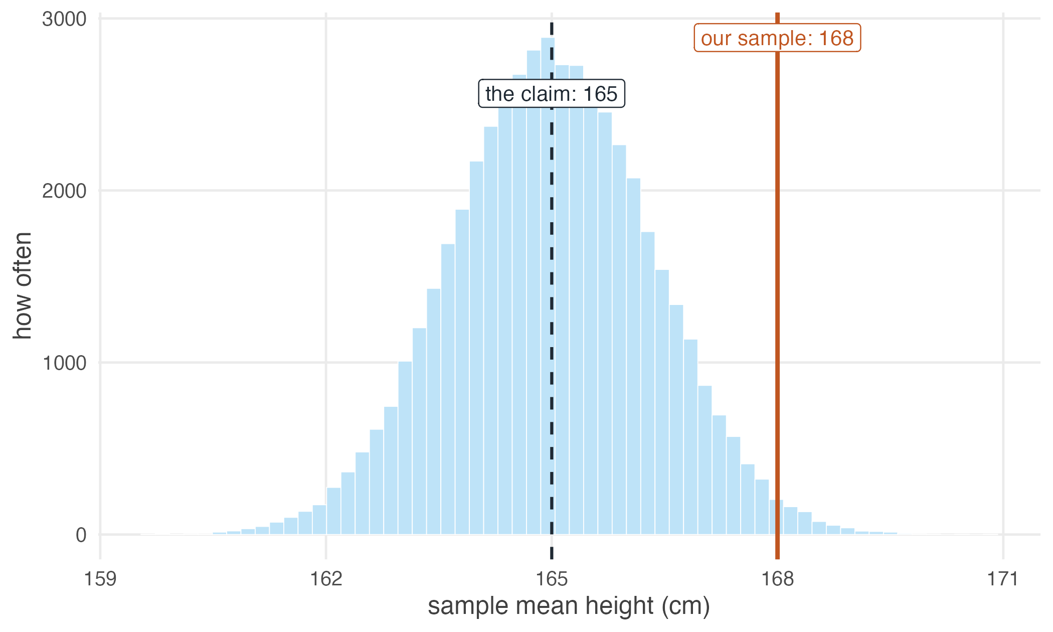
Figure 4.1: Fifty thousand sample means, each from 36 students, drawn from a population whose true mean is 165 cm (dashed line). The solid line marks our observed sample mean of 168 cm. Only about 2.4% of the simulated samples fall at least this far from the claimed value in either direction, which is what makes our sample surprising if the claim is true.