4.5 The worked example, both ways

Back to the students. We have \(\bar{x} = 168\), \(\mu_0 = 165\), \(\sigma = 8\), \(n = 36\), and we will work at \(\alpha = 0.05\).

On paper

Step 1 — Hypotheses.

\[H_0 : \mu = 165 \qquad H_A : \mu \neq 165\]

Step 2 — Critical value. Two-tailed at \(\alpha = 0.05\), so \(Z_{0.025} = 1.96\).

Step 3 — Test statistic.

\[ Z_{calc} = \frac{\bar{x} - \mu_0}{\sigma/\sqrt{n}} = \frac{168 - 165}{8/\sqrt{36}} = \frac{3}{8/6} = \frac{3}{1.333} = 2.25 \]

Step 4 — Decision. \(|2.25| > 1.96\), so we reject \(H_0\) at the 5% level.

Step 5 — The \(p\)-value.

\[ P(|Z| > 2.25) = 2 \times P(Z > 2.25) = 2 \times 0.01222 = 0.0244 \]

If the administration’s claim were true, only 2.4% of samples would sit as far from 165 as ours. That is unlikely enough to reject the claim.

The same thing in R

Now watch every one of those numbers reappear.

xbar  <- 168
mu0   <- 165
sigma <- 8
n     <- 36

se     <- sigma / sqrt(n)          # standard error
z_calc <- (xbar - mu0) / se        # the test statistic
z_crit <- qnorm(1 - 0.05 / 2)      # the critical value
p_val  <- 2 * pnorm(-abs(z_calc))  # the p-value

c(se = se, z_calc = z_calc, z_crit = z_crit, p_value = p_val)

#>      se  z_calc  z_crit p_value 
#> 1.33333 2.25000 1.95996 0.02445

The standard error is 1.3333, the test statistic is 2.25, and the \(p\)-value is 0.0244 — exactly the hand calculation, and near enough exactly the 0.0242 we got by brute-force simulation at the start of the chapter.

Notice what just happened. The simulation, the algebra, and the R code are three descriptions of one idea. The formula is not a rule handed down from above — it is a shortcut for the counting exercise we did by hand in Section 4.1.

And here is the picture the numbers are describing:

plot_rejection(stat = 2.25, crit = 1.96, tails = "two",
               stat_label = "Z = 2.25")

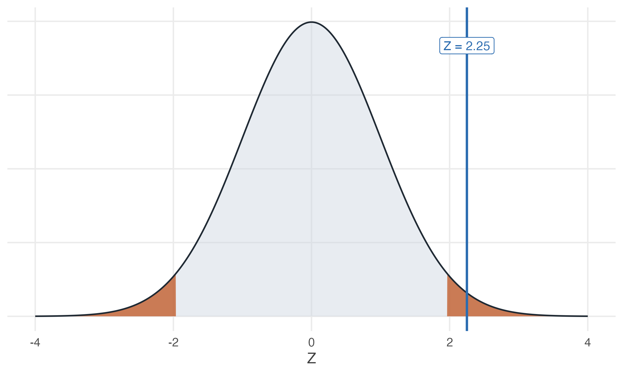
Figure 4.2: The rejection region at \(\alpha = 0.05\) (shaded), with our test statistic of 2.25 falling inside it.

Letting a package do it

For a real dataset rather than summary statistics, z.test() from the BSDA package does the whole thing at once. Since our problem quoted only summary statistics, we first build a sample consistent with them:

library(BSDA)

heights <- make_sample(n = 36, mean = 168, sd = 8)

z.test(heights, mu = 165, sigma.x = 8, conf.level = 0.95)

#> 
#>  One-sample z-Test
#> 
#> data:  heights
#> z = 2.3, p-value = 0.02
#> alternative hypothesis: true mean is not equal to 165
#> 95 percent confidence interval:
#>  165.4 170.6
#> sample estimates:
#> mean of x 
#>       168

Read that output against the hand calculation: z = 2.25, p-value = 0.0244, and a confidence interval that we are about to explain.

z.test() needs sigma.x — the population standard deviation. If you do not know it (and in real work you almost never do), you must not use a \(Z\)-test. Use t.test() instead; see Section 4.7.