3.5 What changes when σ is unknown?
Every interval so far used \(\sigma\). We never know it. Can we just use \(s\) instead?
In the previous section we constructed confidence intervals assuming that the population standard deviation \(\sigma\) was known. This allowed us to calculate the standard error exactly,
\[\mathrm{se}(\bar{X}) = \frac{\sigma}{\sqrt{n}}\]
and to use the normal distribution to determine how far the interval should extend on either side of the sample mean.
In practice the population standard deviation is almost never known. This is not a new problem — Section 3.2 showed how to estimate it with the sample standard deviation \(s\). So a natural question arises.
Can we simply replace \(\sigma\) with \(s\) and continue as before?
At first sight the answer appears to be yes. We replace \(\sigma/\sqrt{n}\) with \(s/\sqrt{n}\) and construct the interval exactly as before.
Unfortunately, that interval is no longer a 95% confidence interval.
Why does the interval change?
The interval developed in the previous section relied on one important fact: the only random quantity in it was the sample mean. The width was fixed, because \(\sigma\) was assumed known.
Once \(\sigma\) is replaced by \(s\), the sample determines both the centre of the interval and its width.
Most samples produce reasonable estimates of the population standard deviation, but some do not. Occasionally a sample happens to contain observations that are unusually similar, giving a value of \(s\) that is too small, and the resulting interval is then narrower than it should be. At the same time, the sample mean may lie further from the population mean than usual.
These two errors can occur together, and when they do the interval is both badly placed and too narrow to reach the truth. The result is that the interval misses more often than we intended.
How serious is the problem?
The easiest way to find out is by simulation.
Suppose the population is normal with mean 26 and standard deviation 5.45. We repeatedly draw samples of size \(n = 10\), estimate the standard deviation with \(s\), and construct intervals in two ways: the first using the familiar normal critical value of 1.96, the second using the appropriate critical value from the \(t\) distribution.
set.seed(6)
n <- 10

cover <- replicate(50000, {
  x  <- rnorm(n, mean = 26, sd = 5.45)
  se <- sd(x) / sqrt(n)
  c(using_1.96       = abs(mean(x) - 26) < 1.96 * se,
    using_t_critical = abs(mean(x) - 26) < qt(0.975, df = n - 1) * se)
})

round(rowMeans(cover), 4)
#> using_1.96 using_t_critical
#> 0.9181 0.9495The results are striking. Using the normal critical value, the interval captures the population mean only about 91.8% of the time rather than the advertised 95%. One statement in twenty was supposed to be wrong; nearly one in twelve is.
Simply replacing \(\sigma\) by \(s\) has made the interval too optimistic.
The \(t\) distribution
To restore the intended coverage we must make the interval slightly wider. This is achieved by replacing the normal critical value with one from Student’s \(t\) distribution, which has heavier tails than the normal.
When \(\sigma\) is unknown, the confidence interval for \(\mu\) is
\[\bar{x} \;\pm\; t_{n-1,\,\alpha/2}\,\frac{s}{\sqrt{n}}\]
where \(t_{n-1,\,\alpha/2}\) is the critical value from the \(t\) distribution with \(n - 1\) degrees of freedom.
In R: qt(1 - alpha/2, df = n - 1).
Notice that the same quantity \(n - 1\) appears here as in the definition of the sample variance. Both arise for the same reason: the sample standard deviation is itself estimated from the data, and estimating the centre used up one observation’s worth of information.
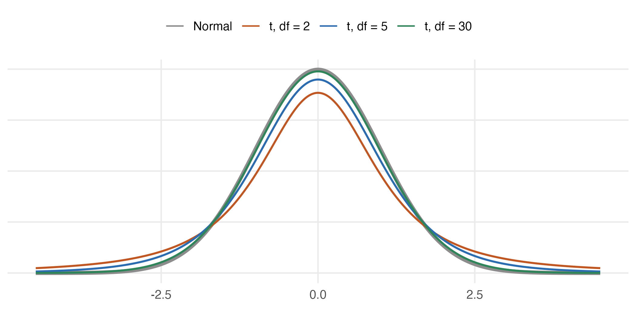
Figure 3.3: The t distribution against the normal. Lower degrees of freedom put more probability in the tails, which is what widens the interval.
The heavier tails are the whole mechanism. Because more of the \(t\) distribution’s probability sits far from the centre, reaching 95% of it requires travelling further — and travelling further is exactly what widens the interval.
How much difference does it make?
The \(t\) distribution depends on the sample size. Small samples carry greater uncertainty about the population standard deviation and therefore need wider intervals. As the sample grows, \(s\) becomes a more reliable estimate of \(\sigma\), the \(t\) distribution approaches the normal, and the difference between the two intervals gradually disappears.
ns <- c(5, 10, 20, 30, 60, 120)
round(data.frame(n = ns, df = ns - 1,
                 t_critical = qt(0.975, ns - 1),
                 z_critical = 1.96,
                 pct_wider  = 100 * (qt(0.975, ns - 1) / 1.96 - 1)), 2)
#> n df t_critical z_critical pct_wider
#> 1 5 4 2.78 1.96 41.66
#> 2 10 9 2.26 1.96 15.42
#> 3 20 19 2.09 1.96 6.79
#> 4 30 29 2.05 1.96 4.35
#> 5 60 59 2.00 1.96 2.09
#> 6 120 119 1.98 1.96 1.03For a sample of five the correction is substantial — the interval is over 40% wider than the normal one. By the time the sample reaches around a hundred observations the two critical values are almost identical, which is why the distinction is rarely important in large samples and matters a great deal in a study with thirty.
One final point
The \(t\) distribution corrects only for the fact that the population standard deviation is unknown.
It does not correct for departures from normality.
If the underlying population is strongly non-normal and the sample is very small, even the \(t\) interval may fall short of its advertised coverage. Repeat the coverage experiment above on the real attendance data rather than a normal population, and at \(n = 10\) the \(t\) interval achieves about 90% rather than 95%. That remaining shortfall has nothing to do with estimating \(\sigma\). It is the sampling distribution of the sample mean not yet being well approximated by a normal distribution.
Two separate issues are in play, and only one of them has been fixed here.
- Estimating an unknown standard deviation — addressed by the \(t\) distribution.
- Approximating the sampling distribution by a normal — addressed by the Central Limit Theorem, and only when \(n\) is large enough for the population in question.
Keeping these distinct is essential for knowing when a confidence interval can be trusted. A \(t\) interval computed from twelve observations of a heavily skewed variable is not made trustworthy by the \(t\) correction; the correction was never aimed at that problem.