6.2 The population regression function

What exactly is regression trying to estimate?

The previous section argued that regression asks a different question from a two-sample comparison. The natural next question is: what is the object we are trying to estimate?

It is tempting to think that regression is trying to draw a straight line through a cloud of points. That is not quite right.

Start with the individual outcomes, because they are noisier than students expect.

Forty-nine students in our data attended exactly 25 classes. They did not receive the same semester GPA.

at25 <- students[students$attendance == 25, ]

round(c(n = nrow(at25), average_gpa = mean(at25$sem_gpa),
        lowest = min(at25$sem_gpa), highest = max(at25$sem_gpa)), 3)

#>           n average_gpa      lowest     highest 
#>      49.000       6.098       1.575       9.075

One scored 1.58 and another 9.08, and forty-seven others lay in between — all of them having attended the same twenty-five classes. Attendance alone plainly does not determine anyone’s grade.

So a line through the individual points cannot be what we are looking for. There is no line that passes near 1.58 and 9.08 at the same value of \(x\).

Instead of looking at every individual student, suppose we ask a different question:

Among students who attended 25 classes, what is the average GPA?

Now repeat the exercise for students who attended 26 classes, then 27, then 28, and so on.

Those averages are called conditional means, because they average GPA conditional on a particular attendance level. We write the conditional mean as

\[E(Y \mid X = x)\]

which simply means “the average value of \(Y\) among all members of the population whose \(X\) equals \(x\).”

The table below approximates these conditional means by grouping attendance into bands.

students$band <- cut(students$attendance,
                     breaks = c(0, 20, 24, 27, 30, 33),
                     labels = c("2–20", "21–24", "25–27", "28–30", "31–32"))

aggregate(sem_gpa ~ band, data = students,
          function(x) round(c(n = length(x), mean_gpa = mean(x)), 2))

#>    band sem_gpa.n sem_gpa.mean_gpa
#> 1  2–20     94.00             4.38
#> 2 21–24     85.00             6.18
#> 3 25–27    155.00             6.30
#> 4 28–30    209.00             6.98
#> 5 31–32    137.00             7.67

Two patterns immediately emerge.

First, students with the same attendance still obtain very different grades. Attendance is therefore not enough to predict an individual’s GPA.

Second, the average GPA rises steadily as attendance increases — from 4.38 to 7.67. Individual outcomes are noisy, but the centre of the distribution shifts upwards.

Regression is interested in this second pattern.

If we computed the conditional mean for every possible attendance level and plotted those averages, we would obtain a curve describing how the average GPA changes with attendance throughout the population.

That curve is called the population regression function (PRF):

\[\text{PRF} \;=\; E(Y \mid X = x)\]

The population regression function is therefore not a fitted line. It exists whether or not we ever estimate it. It is simply the true relationship between attendance and the population’s average GPA.

Figure 6.1 illustrates the idea. The grey points are individual students. The orange points are estimates of the conditional mean within each attendance band. Regression is concerned with those averages, not with explaining every individual observation.

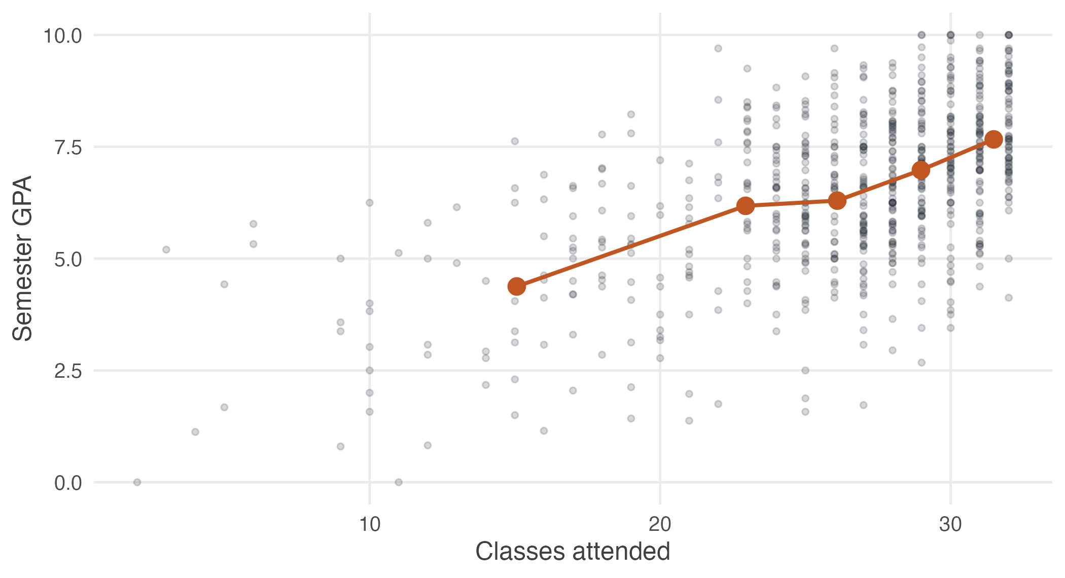
Figure 6.1: Semester GPA against attendance for 680 students. Grey points are individual students; orange points are the average GPA within each attendance band. Regression describes the orange points.

Each conditional mean \(E(Y \mid X = x)\) is a function of \(x\), so the PRF is also called the conditional expectation function (CEF):

\[E(Y \mid X = x) = f(x)\]

The CEF tells us how the average value of \(y\) changes with \(x\). It does not say that \(y = \beta_0 + \beta_1 x\) for every member of the population.

Individual students depart from the average for their attendance level, often by a great deal. Confusing the conditional mean with the individual outcome is the most common misreading of a regression.

Notice that the orange points do not lie exactly on a straight line. Nothing in the definition of the population regression function requires linearity. The conditional mean could be curved, flat over some ranges, or highly nonlinear.

Only now do we make a modelling choice.

The PRF is the object we want to estimate. Unfortunately it is an unknown function, and functions can take infinitely many shapes. To make estimation possible at all, we approximate it with a simple mathematical form.

In this unit we assume that the population regression function is approximately linear,

\[E(Y \mid X = x) = \beta_0 + \beta_1 x\]

because a straight line is simple to estimate, easy to interpret, and often provides a useful approximation to more complicated relationships.

Whether a straight line is a good approximation is an empirical question rather than a mathematical one. Section 7.2 returns to how well it performs for these data.

The population regression function gives us the target. Two questions remain.

First, why do individual students differ from the conditional mean? Second, how can we estimate the population regression function when we observe only a sample rather than the entire population?

The next two sections answer those questions.