7.1 Deriving the estimators

Which values of \(\hat{\beta}_0\) and \(\hat{\beta}_1\) make the sum of squared residuals as small as possible?

Recall the criterion from Section 6.7. We choose \(\hat{\beta}_0\) and \(\hat{\beta}_1\) to minimise

\[L = \sum_{i=1}^{n} \hat{u}_i^2 = \sum_{i=1}^{n}\left(y_i - \hat{\beta}_0 - \hat{\beta}_1 x_i\right)^2\]

This is a minimisation problem in two variables, and it is solved the usual way: differentiate with respect to each, set both derivatives to zero, and solve the pair of equations that results. Those two equations are called the normal equations.

Minimising \(L\) means setting both partial derivatives to zero.

With respect to the intercept:

\[ \begin{aligned} \frac{\partial L}{\partial \hat{\beta}_0} &= \sum_{i=1}^{n} -2\left(y_i - \hat{\beta}_0 - \hat{\beta}_1 x_i\right) = 0 \\[4pt] 0 &= \sum_{i=1}^{n} y_i - n\hat{\beta}_0 - \hat{\beta}_1\sum_{i=1}^{n} x_i && \text{divide by } -2 \text{ and expand} \\[4pt] 0 &= n\bar{y} - n\hat{\beta}_0 - \hat{\beta}_1 n\bar{x} && \text{since } \textstyle\sum x_i = n\bar{x} \\[4pt] \hat{\beta}_0 &= \bar{y} - \hat{\beta}_1\bar{x} && \text{divide by } n \text{ and rearrange} \end{aligned} \]

With respect to the slope:

\[ \begin{aligned} \frac{\partial L}{\partial \hat{\beta}_1} &= \sum_{i=1}^{n} -2x_i\left(y_i - \hat{\beta}_0 - \hat{\beta}_1 x_i\right) = 0 \\[4pt] 0 &= \sum x_i y_i - \hat{\beta}_0\sum x_i - \hat{\beta}_1 \sum x_i^2 \\[4pt] 0 &= \sum x_i y_i - \left(\bar{y} - \hat{\beta}_1\bar{x}\right)n\bar{x} - \hat{\beta}_1\sum x_i^2 && \text{substitute } \hat{\beta}_0 \\[4pt] 0 &= \sum x_i y_i - n\bar{x}\bar{y} - \hat{\beta}_1\left(\sum x_i^2 - n\bar{x}^2\right) \\[4pt] \hat{\beta}_1 &= \frac{\sum x_i y_i - n\bar{x}\bar{y}}{\sum x_i^2 - n\bar{x}^2} \end{aligned} \]

Both parts of that fraction can be written more meaningfully. Expanding the numerator,

\[ \begin{aligned} \sum (x_i - \bar{x})(y_i - \bar{y}) &= \sum x_i y_i - \bar{y}\sum x_i - \bar{x}\sum y_i + n\bar{x}\bar{y} \\[4pt] &= \sum x_i y_i - n\bar{x}\bar{y} \end{aligned} \]

and the denominator,

\[\sum (x_i - \bar{x})^2 = \sum x_i^2 - 2\bar{x}\sum x_i + n\bar{x}^2 = \sum x_i^2 - n\bar{x}^2\]

so that

\[\hat{\beta}_1 = \frac{\sum_{i=1}^{n}(x_i - \bar{x})(y_i - \bar{y})}{\sum_{i=1}^{n}(x_i - \bar{x})^2}\]

The OLS estimators are

\[\hat{\beta}_1 = \frac{\sum(x_i - \bar{x})(y_i - \bar{y})}{\sum(x_i - \bar{x})^2} \qquad\qquad \hat{\beta}_0 = \bar{y} - \hat{\beta}_1\bar{x}\]

The slope is the sample covariance of \(x\) and \(y\) divided by the sample variance of \(x\). It answers: when \(x\) is above its mean, is \(y\) also above its mean, and by how much per unit?

That reading explains several things at once.

If \(x\) and \(y\) move together, the numerator is positive and so is the slope. If they move oppositely, it is negative. If they are unrelated, the products cancel and the slope is near zero.

And the denominator explains why \(x\) must vary. If every student attended the same number of classes, \(\sum(x_i - \bar{x})^2 = 0\) and the slope is undefined — there is no way to learn how GPA responds to attendance from data in which attendance never changes. This is the same requirement as Section 1.1: no variation, nothing to learn.

Doing it by hand and in R

x <- students$attendance
y <- students$sem_gpa

b1 <- sum((x - mean(x)) * (y - mean(y))) / sum((x - mean(x))^2)
b0 <- mean(y) - b1 * mean(x)

c(b0 = b0, b1 = b1)

#>    b0    b1 
#> 1.562 0.189

fit <- lm(sem_gpa ~ attendance, data = students)
coef(fit)

#> (Intercept)  attendance 
#>       1.562       0.189

Identical. lm() solves the same two equations.

So \(\hat{\beta}_1 = 0.189\): each additional class attended is associated with about 0.19 of a GPA point. Ten more classes, roughly 1.9 points — which on a ten-point scale is a great deal.

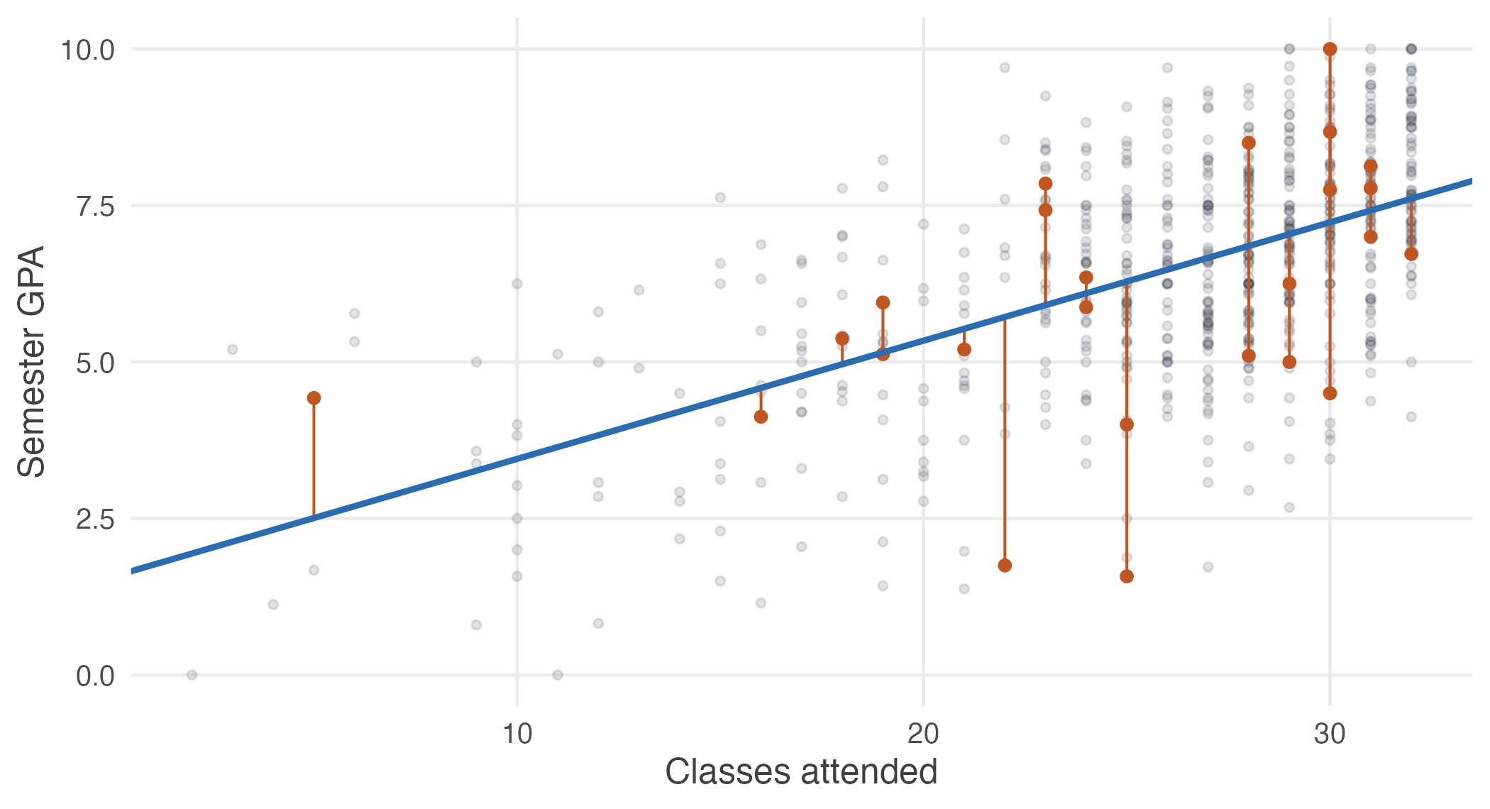
Figure 7.1: The fitted line, with the vertical distances it misses by shown for a handful of students. Ordinary least squares chooses the line making the sum of those squared distances as small as possible.