7.6 When the error variance is not constant

The standard error formula rested on one new assumption. Is it true?

The previous section derived a formula for the standard error, and that derivation needed CLRM5: the errors have the same variance at every value of \(x\).

\[\mathrm{Var}(u \mid x) = \sigma^2 \quad \text{for every } x\]

Read as a claim about the world, that says the unobserved factors are just as spread out among students who attended 5 classes as among those who attended 30, and just as spread out among poor households as among rich ones.

Often they are not.

Consider annual earnings against years of schooling.

Someone with two years of schooling has little scope to be unusual. Their earnings are constrained from above by the work available to them, and there is not much room between the floor and that ceiling.

Someone with sixteen years of schooling might be a clerk, a teacher, a doctor or a company director. The same qualification is consistent with an enormous range of outcomes, because what happens after school depends on far more than school.

So the spread of the errors grows with \(x\). This is heteroskedasticity, and in economic data it is the normal case rather than the exception.

What it looks like

The diagnostic is a residual plot: the residuals against the fitted values. Homoskedasticity appears as a band of roughly constant width, heteroskedasticity as a fan.

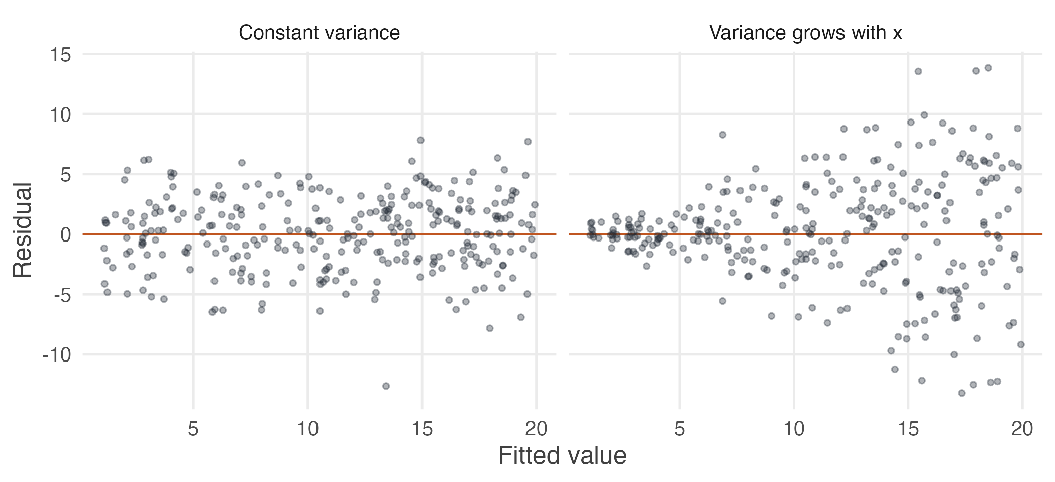
Figure 7.6: Residual plots from two simulated datasets. On the left the error variance is constant and the band has an even width. On the right it grows with x, and the band fans out. This is the shape to look for.

Now the real thing. Regress annual earnings on years of education for the 20,000 wage earners and look at how the residuals are spread.

wages <- read.csv("data/wages-india-synthetic.csv")
fit_w <- lm(annual_earnings ~ education, data = wages)

u_w <- residuals(fit_w)
f_w <- fitted(fit_w)

quartile <- cut(f_w, quantile(f_w, 0:4/4), include.lowest = TRUE)
round(tapply(u_w, quartile, sd))

#> [2.34e+04,2.88e+04] (2.88e+04,5.04e+04] (5.04e+04,7.19e+04] (7.19e+04,1.04e+05] 
#>               42504               61998               93743              153304

The residuals in the top quarter of fitted values are more than three times as spread out as those in the bottom quarter.

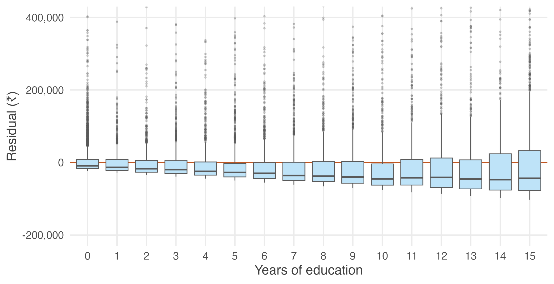
Figure 7.7: Residuals from a regression of annual earnings on years of schooling, shown as a boxplot at each level of education. The boxes widen steadily to the right. A few extreme residuals lie above the range plotted.

Education takes only whole-number values, so a plain scatter of residuals against fitted values collapses into vertical stripes. A box at each level of education shows the same thing more legibly, and the widening is unmistakable.

Formal tests exist. The Breusch–Pagan and White tests both regress squared residuals on the explanatory variables and ask whether anything is there.

They are worth knowing about, and they are not what this book recommends reaching for first. A plot settles the matter faster and tells you the shape of the problem rather than merely announcing its presence — and, as the next section shows, a fan-shaped residual plot sometimes means the functional form is wrong rather than the variance non-constant. A test statistic cannot tell you which.

Does heteroskedasticity matter?

Here is the surprise.

The fitted line is unaffected.

The proof that \(E(\hat{\beta}_1) = \beta_1\) used CLRM1 to CLRM4 and never mentioned CLRM5. The estimate is still centred on the truth, and heteroskedasticity introduces no bias whatever.

The standard error is wrong.

\(\mathrm{Var}(\hat{\beta}_1) = \sigma^2/\text{SST}_x\) was obtained by replacing every \(\mathrm{Var}(u_i)\) with a common \(\sigma^2\). If no common \(\sigma^2\) exists, that step is invalid — and with it the standard errors, the \(t\) statistics, the \(p\)-values and the confidence intervals.

So the coefficient is fine and the reported uncertainty around it is not. That is why this matters: not because the arithmetic of the line changes, but because everything we say about how much to trust the line is computed from a formula that no longer applies.

How wrong?

We can measure it, by simulating from a model where we know both the truth and the severity of the problem.

robust_se <- function(m) {
  X <- model.matrix(m); u <- residuals(m)
  n <- nrow(X); k <- ncol(X)
  XtXi <- solve(crossprod(X))
  V <- XtXi %*% (t(X) %*% diag(u^2) %*% X) %*% XtXi * n / (n - k)
  sqrt(diag(V))[2]
}

set.seed(8)
out <- replicate(4000, {
  x <- rexp(60, rate = 1/5)              # skewed x, as economic data often is
  y <- 2 + 1 * x + rnorm(60, sd = x)     # sd of the error grows with x
  m <- lm(y ~ x)
  c(b1 = coef(m)[2], classical = coef(summary(m))[2, 2], robust = robust_se(m))
})

round(c(actual_sd_of_b1  = sd(out[1, ]),
        avg_classical_se = mean(out[2, ]),
        avg_robust_se    = mean(out[3, ])), 4)

#>  actual_sd_of_b1 avg_classical_se    avg_robust_se 
#>           0.4301           0.1764           0.3293

The true slope is 1. Across four thousand samples \(\hat{\beta}_1\) has a standard deviation of 0.43 — that is the actual variability of the estimator, the thing a standard error is supposed to report.

The classical standard error reports 0.18. Software printing 0.18 is claiming a precision the estimator does not have, by a factor of more than two.

round(c(classical = mean(abs(out[1, ] - 1) < qt(0.975, 58) * out[2, ]),
        robust    = mean(abs(out[1, ] - 1) < qt(0.975, 58) * out[3, ])), 3)

#> classical    robust 
#>     0.588     0.851

This is the finding that matters, and it is worth stating slowly.

A confidence interval advertised as 95% should contain the true slope in roughly 95 of every 100 repeated samples. Here it succeeds 59 times.

The problem is not the estimator. \(\hat{\beta}_1\) is unbiased and behaving exactly as it should. The problem is that we underestimated its variability, and so drew an interval far too narrow around a perfectly good estimate.

Robust standard errors

The repair does not touch \(\hat{\beta}_1\), which needs no repairing. It replaces the formula for the variance with one that does not assume a common \(\sigma^2\), using each observation’s own squared residual in place of a single estimate.

These are called White heteroskedasticity-robust standard errors, after Halbert White’s influential work, and in ordinary conversation simply robust standard errors. All three names refer to the same idea.

Robust standard errors leave the fitted line unchanged. They alter only how the uncertainty around it is calculated.

The coefficients you report are identical either way. What changes is the second column of the output, and everything computed from it.

In the simulation they report 0.33 against a true 0.43, and lift coverage from 59% to 85%. A large improvement, and visibly not a complete repair at this sample size and this severity.

round(c(classical_se = coef(summary(fit_w))[2, 2],
        robust_se    = robust_se(fit_w)), 2)

#>        classical_se robust_se.education 
#>               137.4               175.2

For the earnings regression the robust standard error is 175 against a classical 137 — a quarter larger again. Any conclusion resting on the difference between those two numbers was resting on an assumption the residual plot had already refused.

The calculation above is written out longhand so that nothing is hidden. In practice one reaches for a package.

library(sandwich)   # variance estimators
library(lmtest)     # tests that accept them

coeftest(fit_w, vcov = vcovHC(fit_w, type = "HC1"))

Stata users will recognise the same thing as reg y x, vce(robust).

The variants HC0 through HC3 differ only in how the variance is adjusted for finite samples. HC1 is the most common default and matches Stata’s; for moderate and large samples the choice rarely matters.

White standard errors are the first member of a family, and it is worth knowing that the family exists.

• White (heteroskedasticity-robust) standard errors relax the assumption of constant error variance.
• Cluster-robust standard errors also allow errors to be correlated within groups — students within a school, households within a village.
• HAC or Newey–West standard errors allow correlation across time.

All three estimate the variance of the same OLS estimator in different circumstances. None of them changes the coefficients, and none of them is a different method of regression. They are different answers to the single question of how much the estimator would vary across repeated samples.

Three things robust standard errors do not do.

They do not fix bias. There was none to fix.

They do not fix a wrong functional form. A fan-shaped residual plot sometimes means the relationship is not linear rather than that the variance is non-constant, and robust standard errors would paper over that. A later unit takes this up.

They do not work miracles in small samples, as the simulation shows.

Modern practice is to report robust standard errors by default in cross-sectional work.

This is exactly the logic of Section 5.4. Classical standard errors assume equal variances, as the pooled two-sample \(t\)-test did; robust standard errors relax that assumption, as Welch’s test did. In both cases the relaxed version costs very little when the assumption holds and protects you when it does not — and in both cases the assumption can never be established, only left un-rejected.

The wider lesson

Heteroskedasticity is a good example of a broader principle, and the principle is worth more than the topic.

Regression coefficients answer one question: what is the relationship?

Standard errors answer another: how sure are we?

The first can be correct while the second is badly wrong.

Students often assume that if a regression is right, everything about it is right. This section is the first place where that fails cleanly — the line is unbiased, the residuals sum to zero, \(R^2\) is computed correctly, and the confidence interval still misses the truth two times in five.

Estimation and inference are separate problems, and they can fail separately.