2.2 When can a sample represent a population?

Before comparing estimators — can a sample tell us anything about a population at all?

There is an objection to deal with first. Everything above assumed that a sample carries information about the population it came from. That is not automatic. It depends on how the sample was collected, and it can fail badly.

Rather than assert this, we can watch it happen. Below is a population of 20,000 households, spread across 200 localities. Sixty of those localities are urban, and incomes there are higher. Because we build the population ourselves, we know its mean exactly.

set.seed(2)

n_loc <- 200                 # localities
per   <- 100                 # households in each

urban    <- rep(c(TRUE, FALSE), times = c(60, 140))
loc_mean <- 18000 + 9000 * urban + rnorm(n_loc, sd = 4000)

pop <- data.frame(
  locality = rep(1:n_loc, each = per),
  urban    = rep(urban,   each = per),
  income   = round(rnorm(n_loc * per, rep(loc_mean, each = per), sd = 5000))
)

mu    <- mean(pop$income)
sigma <- sd(pop$income)

c(mu = mu, sigma = sigma, se_if_random = sigma / sqrt(100))

#>           mu        sigma se_if_random 
#>      20724.8       7974.4        797.4

The population mean is 20,725. Each survey below collects 100 households, and is repeated a thousand times. Only the method of collection differs.

# Survey A: 100 households drawn at random from the whole population
# Survey B: 100 households drawn at random, but only from urban localities
# Survey C: five localities chosen at random, 20 households in each
# Survey D: five *urban* localities chosen at random, 20 households in each

cluster_sample <- function(pool) {
  chosen <- sample(pool, 5)
  unlist(lapply(chosen, function(l) sample(pop$income[pop$locality == l], 20)))
}

urban_pop <- pop$income[pop$urban]
urb_loc   <- which(urban)

set.seed(11)
designs <- list(
  A = replicate(1000, mean(sample(pop$income, 100))),
  B = replicate(1000, mean(sample(urban_pop,  100))),
  C = replicate(1000, mean(cluster_sample(1:n_loc))),
  D = replicate(1000, mean(cluster_sample(urb_loc)))
)

round(t(sapply(designs, function(x) c(centre = mean(x), spread = sd(x)))))

#>   centre spread
#> A  20702    788
#> B  27503    667
#> C  20774   2843
#> D  27538   2140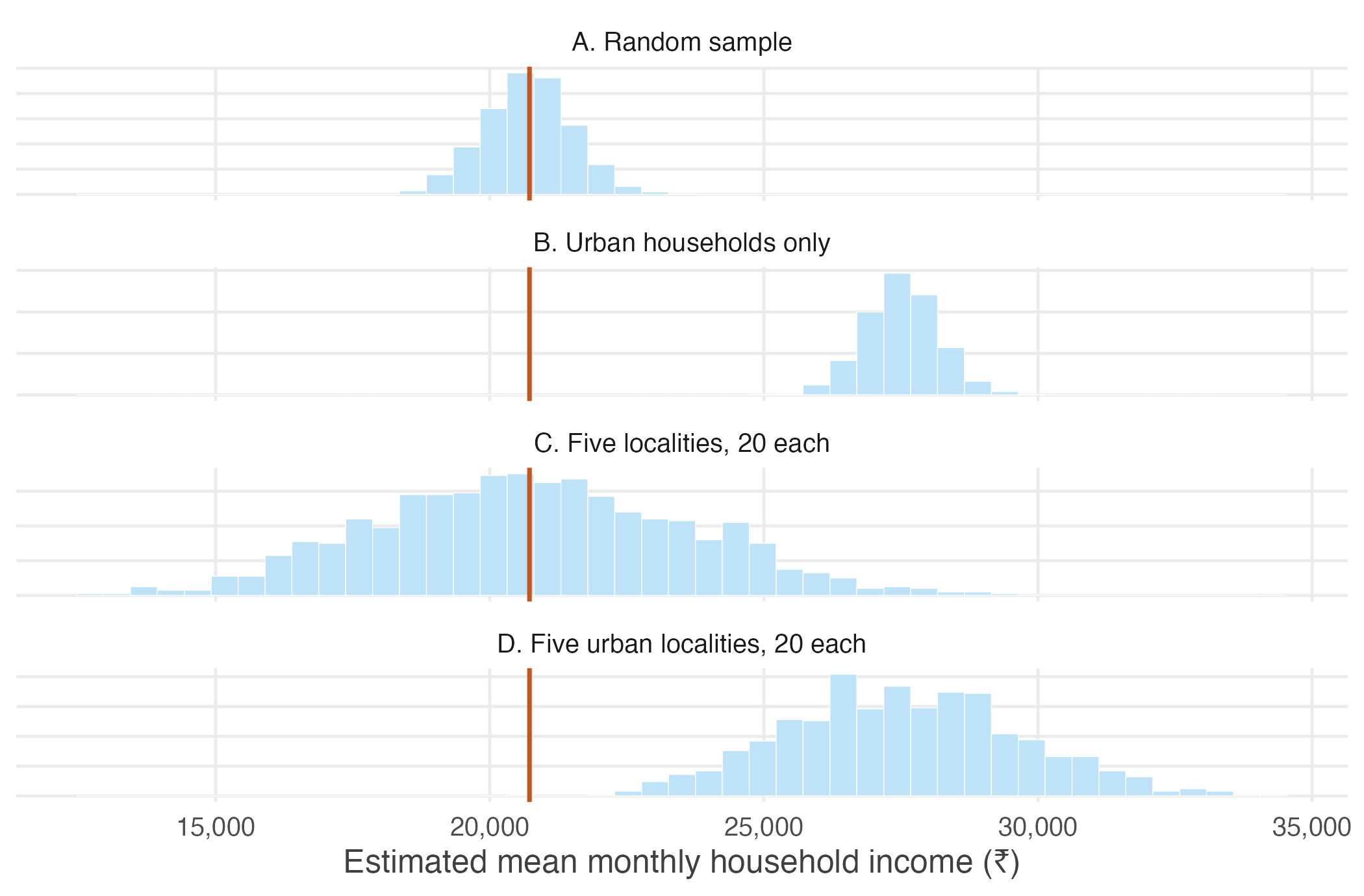

Figure 2.1: One thousand surveys under each design. The vertical line is the true population mean. Only the first design is both centred on it and as precise as theory promises.

Read the four rows carefully, because they fail in different ways.

Survey A works. The thousand estimates are centred on the population mean, and their spread is almost exactly the \(\sigma/\sqrt{n}\) predicted in the previous unit.

Survey B is wrong, and looks excellent. Every estimate is far too high — the surveyor never visits a village, so village incomes cannot appear in the answer. Notice the second column: the spread is smaller than in Survey A. Urban households resemble one another, so the estimates agree closely with each other while agreeing on the wrong number. Consistency is not accuracy. This is the more dangerous failure, because a narrow spread is easily mistaken for a reliable result.

Survey C is centred correctly but far too variable. Choosing five localities and surveying twenty households in each is cheap and common — an interviewer travels to a place and works through it. But households in a locality resemble one another, so the second household adds much less new information than the first. The sample has 100 rows and nothing like 100 households’ worth of information. The spread is over three times what \(\sigma/\sqrt{n}\) predicts, so a researcher using that formula would report confidence they have not earned.

Survey D fails both ways at once, which is what most convenience samples do in practice.

What did the first survey have that the others did not?

Two things, and each failure above corresponds to losing one of them.

Identically distributed — every observation is drawn from the same distribution, and it is the distribution we want to learn about. Survey B violated this: urban households are drawn from a different distribution than the population of Indian households.

Independent — knowing the value of one observation tells us nothing about another. Survey C violated this: neighbours share a locality, a labour market and often an occupation.

Together the two are abbreviated i.i.d.

These assumptions are not mathematical decoration. Sections 2.4 and 2.5 derive the two properties that justify using the sample mean, and each derivation uses exactly one of them — in one identifiable line. Break the assumption and the property it supports disappears, which is precisely what the four surveys show.

No amount of mathematical sophistication repairs a badly collected sample. If the households you surveyed are not drawn from the population you are asking about, there is no formula that recovers the ones you missed.

Good inference begins with study design, not with statistics.