8.3 What does “holding constant” actually mean?

Nothing in the data was held anywhere. So what does the regression do?

The phrase holding other variables constant is used constantly in economics. It is also one of the least understood.

Nothing in the data was actually held fixed. Every student has a different attendance, a different prior GPA and a different admission score. Nobody reran the semester while changing only one variable.

So what does the regression actually do?

Predicting attendance

The answer can be described as a simple two-step procedure.

1. Predict attendance using the control variables.
2. Keep only what cannot be predicted.
3. Ask whether that remaining variation predicts grades.

Take the first step slowly, because everything rests on it.

Imagine predicting every student’s attendance using only their previous GPA and admission score. Some students attend exactly as much as we would expect. Some attend much more. Some attend much less.

Those unexpected differences are the residuals.

step1 <- lm(attendance ~ cum_gpa + admission_score, data = students)
r1    <- residuals(step1)

round(c(r2_of_step1      = summary(step1)$r.squared,
        cor_with_cumgpa  = cor(r1, students$cum_gpa),
        cor_with_admscr  = cor(r1, students$admission_score)), 4)

#>     r2_of_step1 cor_with_cumgpa cor_with_admscr 
#>          0.2906          0.0000          0.0000

Prior GPA and admission score together account for 29% of the variation in attendance. The residual carries the rest, and it is uncorrelated with both — to machine precision, because that is what least squares guarantees.

That last point is the one that matters. Whatever these residuals contain, they contain nothing about prior GPA or admission score.

Using only what could not be predicted

Now regress semester GPA on that residual alone.

step2 <- lm(students$sem_gpa ~ r1)

noquote(format(c(from_two_steps   = unname(coef(step2)[2]),
                 from_lm_directly = unname(coef(full)["attendance"])),
               digits = 10))

#>   from_two_steps from_lm_directly 
#>     0.1360121381     0.1360121381

The same number, to ten significant figures.

This result is known as the Frisch–Waugh–Lovell theorem, and it holds for every coefficient in every multiple regression, not just this one.

Multiple regression does not compare students with the same attendance.

It compares students who differ in the part of attendance that cannot already be explained by the other variables.

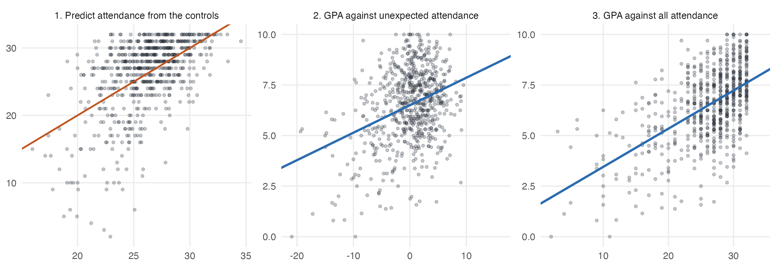
Figure 8.1: The two steps, and what they change. Panel 1 predicts attendance from prior GPA and admission score; the orange line is where a student would sit if the prediction were exact, and the vertical distances from it are the residuals. Panel 2 regresses GPA on those residuals alone. Panel 3 regresses GPA on attendance itself. The horizontal axes in panels 2 and 3 are drawn to the same width, so the two slopes can be compared directly.

Two students with the same prior GPA and admission score are predicted to attend roughly the same number of classes.

If one attends more than predicted and the other less, that difference is unrelated to the observed controls.

Multiple regression asks whether those unexpected differences in attendance are associated with differences in grades.

Why the coefficient changes

The coefficient changes because the variation changes.

The simple regression used all the variation in attendance — the third panel of the figure. The multiple regression uses only the part that prior record cannot account for — the second panel. Those are different questions asked of different variation, and there is no reason for them to give the same answer.

This is worth separating from the more familiar account, which says that controls remove bias. They may well do so, and Section 8.7 takes that up. But the mechanism is not that something contaminating has been subtracted from the answer. It is that the estimator is now working with a different set of comparisons.

Why the standard error usually grows

The residual \(\hat{r}_1\) has less spread than attendance itself: a standard deviation of 4.6 classes against 5.5.

round(c(sd_of_attendance = sd(students$attendance),
        sd_of_residual   = sd(r1)), 3)

#> sd_of_attendance   sd_of_residual 
#>            5.455            4.595

Section 7.5 established that the precision of a slope depends on the spread of the explanatory variable. Discarding variation must therefore cost something, and Section 8.4 works out the bill.

That is the trade the whole method rests on. A control buys a narrower, more credible comparison, and pays for it in precision.