2.3 How can we judge an estimator?

If \(\mu\) is never known, how can we ever tell whether an estimator is any good?

We now know what a sample must satisfy. The original question remains: of the many rules available, why the sample mean?

The obstacle is the one identified at the start. To see whether an estimator lands near the truth we would have to know the truth, and in any real application we do not. If we survey Indian households we do not know true average household income; if we sample firms we do not know true average productivity. There is nothing to compare against.

The way around this is to build a laboratory. We construct one artificial population whose properties are known exactly, and study repeated sampling from it. Because the true mean is known in advance, every sample mean can be measured against it. Nothing is being discovered about the world here — the point is to watch a procedure work under conditions where its performance is visible.

The population

Take a deck of playing cards, scored A = 1, J = 11, Q = 12, K = 13, and 2 through 10 at face value.

deck <- rep(1:13, times = 4)

c(N = length(deck), mu = mean(deck), sigma = sd(deck))

#>      N     mu  sigma 
#> 52.000  7.000  3.778

This population contains 52 values. Its mean is exactly \(\mu = 7\) and its standard deviation is \(\sigma = 3.78\). Both are known with certainty, which is exactly what real data never offers.

One sample from it

Draw ten cards and compute their average.

set.seed(7)
mean(sample(deck, size = 10, replace = TRUE))

#> [1] 5.7

The result is not 7. Draw again and it would differ again — sampling variation, as before. What is new is that we can see how far this sample strayed, because we know where it should have been.

Note replace = TRUE: each card is returned to the deck before the next draw.

That is what makes the draws independent, in the sense of the previous section. Drawing without replacement changes what remains after each card is removed, so the draws are dependent and the sample mean varies slightly less than theory predicts.

It is also the better model of what we usually mean. Surveying 2,000 people does not meaningfully deplete a population of a billion.

A thousand samples

One sample tells us little about a procedure. Repeating the exercise a thousand times shows the whole sampling distribution — and, for the first time, shows it alongside the truth it is supposed to be tracking.

set.seed(7)
deck_means <- replicate(1000, mean(sample(deck, size = 10, replace = TRUE)))

c(mean_of_sample_means = mean(deck_means),
  sd_of_sample_means   = sd(deck_means))

#> mean_of_sample_means   sd_of_sample_means 
#>                6.932                1.201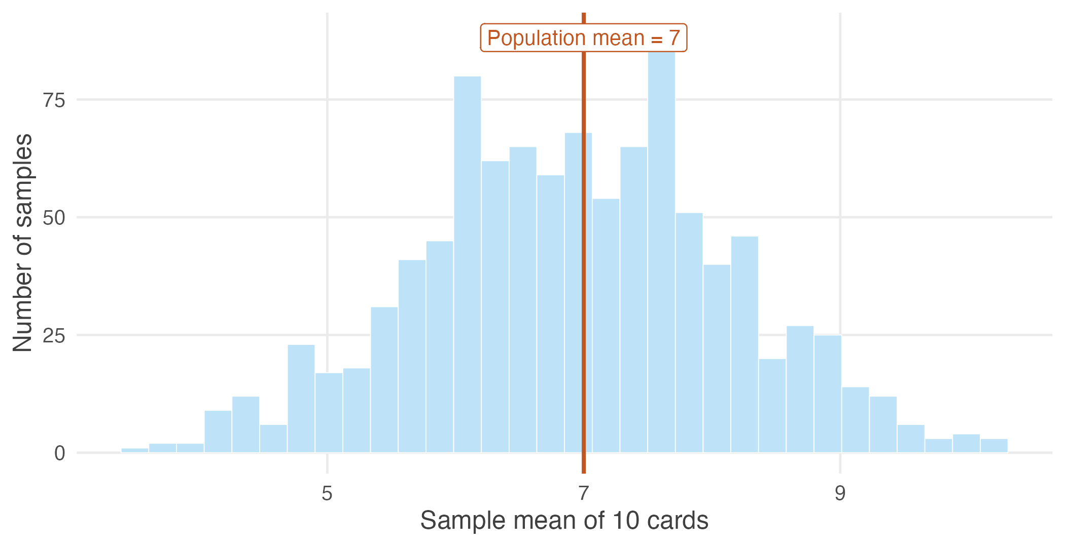

Figure 2.2: One thousand sample means, each computed from 10 cards drawn from a population whose mean is exactly 7.

Two features of this picture are worth separating, and the next two sections take them one at a time: where the distribution sits, and how wide it is.