4.7 When σ is unknown: the t-test

Everything so far assumed we knew the population standard deviation \(\sigma\). We almost never do.

Everything else stays the same. We still compare the sample mean with the value the null hypothesis claims, and we still ask how surprising that gap would be if the claim were true. The only change is that we must first estimate \(\sigma\) from the sample itself.

That estimate is not free. Replacing \(\sigma\) with the sample standard deviation \(s\) adds a second source of uncertainty, and the statistic

\[t_{calc} = \frac{\bar{x} - \mu_0}{s/\sqrt{n}}\]

no longer follows a normal distribution. It follows Student’s \(t\) with \(n - 1\) degrees of freedom — a distribution with fatter tails, which demands more evidence before it will let you reject.

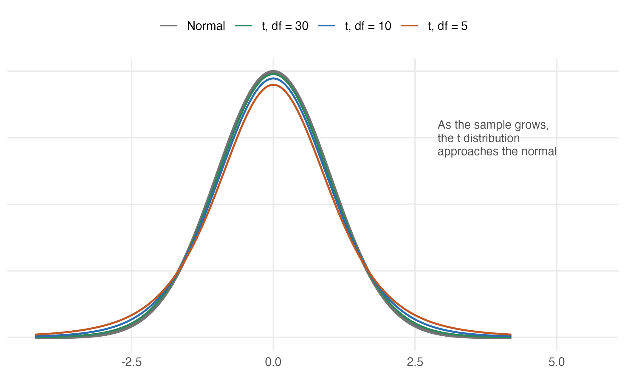
Figure 4.4: Student’s t against the standard normal. Fewer degrees of freedom put more probability in the tails, so critical values sit further out and more evidence is needed to reject. By 30 degrees of freedom the two are already hard to tell apart.

Settling the question with the actual class

We opened this chapter with a made-up sample of 36 students. We can now do the real thing. stats-class.csv holds the survey this class filled in — names, ages, heights, gender:

students <- read.csv("data/stats-class.csv")

str(students)

#> 'data.frame':    33 obs. of  4 variables:
#>  $ student_id: chr  "S01" "S02" "S03" "S04" ...
#>  $ age       : int  31 19 18 18 19 18 18 21 18 19 ...
#>  $ height    : int  178 161 181 164 170 175 176 186 161 170 ...
#>  $ gender    : chr  "M" "F" "M" "F" ...

Thirty-three rows, but look at the last one. One student left age and height blank, and another did not give a gender:

students[!complete.cases(students), ]

#>    student_id age height gender
#> 8         S08  21    186   <NA>
#> 33        S33  NA     NA      F

Working with real data. What follows is not part of hypothesis testing. It is the sort of thing that has to be dealt with the moment you leave textbook datasets behind, and this is the first point in the book where you have.

A blank is not always an NA. In a numeric column an empty field is read as NA, but in a text column it is read as the empty string "" — and "" is a perfectly ordinary value as far as is.na(), complete.cases() and na.rm are concerned. A gap in a text column can therefore hide in plain sight.

If a dataset you did not prepare yourself has blanks, say so explicitly when you read it:

read.csv("somefile.csv", na.strings = c("", "NA"))

The files in this book are already written so that plain read.csv() does the right thing.

mean() returns NA if even one value is missing — it refuses to guess what you meant. Pass na.rm = TRUE to drop the gaps, and always know how many you dropped.

mean(students$height)                  # NA — one height is missing

#> [1] NA

mean(students$height, na.rm = TRUE)    # 32 students

#> [1] 169.5

Now the test. We do not know the population standard deviation of student heights, so this is a \(t\)-test, not a \(Z\)-test:

heights_real <- students$height[!is.na(students$height)]

c(n = length(heights_real),
  mean = mean(heights_real),
  sd = sd(heights_real))

#>      n   mean     sd 
#>  32.00 169.50   8.71

t.test(heights_real, mu = 165)

#> 
#>  One Sample t-test
#> 
#> data:  heights_real
#> t = 2.9, df = 31, p-value = 0.006
#> alternative hypothesis: true mean is not equal to 165
#> 95 percent confidence interval:
#>  166.4 172.6
#> sample estimates:
#> mean of x 
#>     169.5

\(t = 2.92\) on 31 degrees of freedom, with a \(p\)-value of 0.0064. We reject the claim that the average is 165 cm. The 95% interval, \([166.4,\ 172.6]\), excludes 165 — the same verdict, as always.

Notice how much narrower this is than the textbook version of the problem. The opening example assumed we somehow knew \(\sigma = 8\). Here we had to estimate it from 32 people, and the \(t\) distribution charges us for that uncertainty with a wider interval and a higher bar to clear.

Statistical validity is not sampling validity. Notice what the data is not: 32 students in one classroom are not a random sample of all APU students.

Every number above is correctly computed. The \(t\) statistic, the degrees of freedom, the \(p\)-value and the interval are all exactly right for this sample. Whether they answer a question about the university is a separate matter, and a harder one — and no amount of care with the arithmetic addresses it. The formulas cannot tell you which population you were sampling from; only the design can.

Worked example

The dean estimates that full-time faculty teach 11.0 classroom hours per week. You sample eight faculty members. Can you reject the dean’s claim at \(\alpha = 0.10\)? At \(\alpha = 0.01\)?

hours <- c(11.8, 8.6, 10.5, 7.9, 6.4, 10.4, 10.0, 8.2)

c(n = length(hours), mean = mean(hours), sd = sd(hours))

#>     n  mean    sd 
#> 8.000 9.225 1.749

Before calculating anything, form an expectation.

The claim is 11.0 hours and the sample averages 9.2 — a gap of nearly two hours. But there are only eight faculty members, and their hours range from 6.4 to 11.8, so the sample is both small and quite spread out.

Do you expect to reject the claim at the 10% level? At the 1%? Commit to an answer before reading on, and then see whether the arithmetic agrees.

On paper. With \(\bar{x} = 9.225\), \(s = 1.749\), \(n = 8\) and \(df = 7\):

\[ t_{calc} = \frac{9.225 - 11}{1.749/\sqrt{8}} = \frac{-1.775}{0.618} = -2.87 \]

The critical values are \(t_{0.05,\,7} = 1.895\) and \(t_{0.005,\,7} = 3.499\).

• At \(\alpha = 0.10\): \(2.87 > 1.895\) \(\Rightarrow\) reject \(H_0\).
• At \(\alpha = 0.01\): \(2.87 < 3.499\) \(\Rightarrow\) fail to reject \(H_0\).

In R. Both the pieces and the packaged version:

t_calc <- (mean(hours) - 11) / (sd(hours) / sqrt(length(hours)))
t_crit <- qt(c(0.95, 0.995), df = 7)     # 10% and 1%, two-tailed

c(t_calc = t_calc, crit_10pct = t_crit[1], crit_1pct = t_crit[2])

#>     t_calc crit_10pct  crit_1pct 
#>     -2.870      1.895      3.499

t.test(hours, mu = 11, conf.level = 0.90)

#> 
#>  One Sample t-test
#> 
#> data:  hours
#> t = -2.9, df = 7, p-value = 0.02
#> alternative hypothesis: true mean is not equal to 11
#> 90 percent confidence interval:
#>   8.053 10.397
#> sample estimates:
#> mean of x 
#>     9.225

The \(p\)-value is 0.024 — below 0.10 but above 0.01, exactly matching the two different verdicts we reached by hand.

The same data can be “significant” at one level and not at another. Nothing has changed about the world between those two lines — only how much risk of a false alarm we were willing to tolerate. This is why reporting the \(p\)-value itself is far more informative than reporting a bare “significant / not significant.”