9.3 Elasticities: weight and fuel efficiency

What does the log–log form buy us on the cars?

level_level <- lm(mileage_kmpl ~ weight_kg, data = cars)
log_log     <- lm(log(mileage_kmpl) ~ log(weight_kg), data = cars)

round(rbind(level_level = c(slope     = coef(level_level)[2],
                            r_squared = summary(level_level)$r.squared),
            log_log     = c(slope     = coef(log_log)[2],
                            r_squared = summary(log_log)$r.squared)), 4)

#>             slope.weight_kg r_squared
#> level_level         -0.0060    0.6515
#> log_log             -0.8252    0.7136

The log–log slope is \(-0.825\): a car that is 1% heavier is about 0.83% less fuel-efficient.

That is a sentence anyone can evaluate, and — unlike \(-0.00601\) — it would be unchanged if weight were recorded in tonnes.

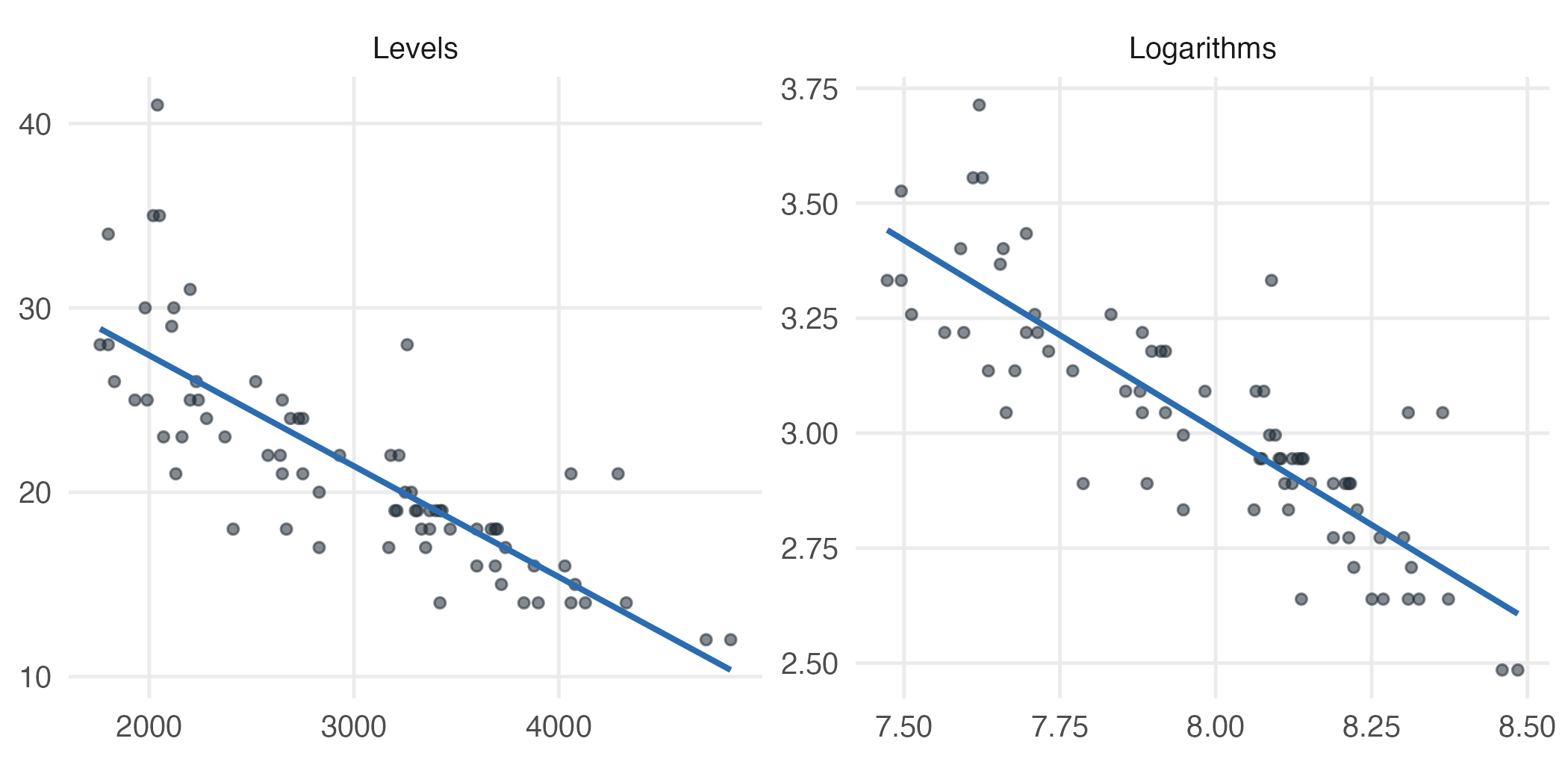
Figure 9.1: The same 74 cars in levels and in logarithms. Both look broadly linear; the logarithmic version is a little tighter around the line, which is the improvement in R-squared from 0.65 to 0.71. The gain here is real but modest – the case for the log form rests mainly on interpretation.

The fit also improves, from \(R^2 = 0.65\) to \(0.71\). That is a modest gain rather than a dramatic one, and the case for the log form here rests mainly on interpretation. Still, the direction is not an accident: a constant proportional penalty for weight describes cars better than the constant absolute penalty the level–level model imposed.

A great deal of weak empirical work consists of fitting a straight line to a relationship that is not straight, and reporting the slope as though it described the whole range.

The residual plot of Section 7.6 catches this: a curved band of residuals means the functional form is wrong, not that the variance is non-constant.

Fitting a line is a choice. Check it.