8.6 Testing several coefficients at once
We can test one coefficient. Why not just do it repeatedly?
Suppose we want to know whether prior record matters at all — whether prior GPA and admission score, taken together, belong in the model.
\[H_0 : \beta_2 = 0 \;\text{ and }\; \beta_3 = 0\]
The obvious approach is two \(t\)-tests. It does not work, and seeing why is more useful than the test that replaces it.
Why separate tests fail
Each \(t\)-test asks about one coefficient while the others stay in the model. The joint null asks about both coefficients simultaneously. These are different claims, and they can disagree.
Here is a small constructed example where the disagreement is stark. Two explanatory variables both genuinely affect \(y\), and they are highly correlated with each other.
set.seed(11)
n  <- 60
z  <- rnorm(n)
x1 <- z + rnorm(n, sd = 0.25)
x2 <- z + rnorm(n, sd = 0.25)
y  <- 1 + 0.8 * x1 + 0.8 * x2 + rnorm(n, sd = 2)

round(cor(x1, x2), 3)
#> [1] 0.912#> Estimate Std. Error t value Pr(>|t|)
#> (Intercept) 1.0765 0.2577 4.177 0.0001
#> x1 0.9376 0.7197 1.303 0.1979
#> x2 0.7246 0.6890 1.052 0.2974Neither variable is close to significant. The \(p\)-values are 0.20 and 0.30, and a reader taking each test at face value would drop both.
Now test them together.
#> Analysis of Variance Table
#>
#> Model 1: y ~ 1
#> Model 2: y ~ x1 + x2
#>   Res.Df RSS Df Sum of Sq    F    Pr(>F)
#> 1     59 334
#> 2     57 216  2       119 15.7 0.0000038 ***
#> ---
#> Signif. codes:  0 '***' 0.001 '**' 0.01 '*' 0.05 '.' 0.1 ' ' 1
Jointly, they are overwhelmingly significant.
There is no contradiction, and the resolution is Section 8.3.
The \(t\)-test on \(x_1\) uses only the part of \(x_1\) that is unrelated to \(x_2\). Since the two are correlated at 0.91, almost nothing is left, and that remainder tells us very little. The same is true of \(x_2\).
The data cannot say which of the two is responsible. They are perfectly clear that one of them is.
Two individually insignificant coefficients therefore do not license dropping both. What can be said about them separately, and what can be said about them together, are different things.
The restricted and unrestricted models
The joint test compares two models.
The unrestricted model is the one we believe might be appropriate:
\[y = \beta_0 + \beta_1 x_1 + \cdots + \beta_k x_k + u\]
The restricted model is what remains after imposing the null. If the null sets \(q\) coefficients to zero, the restricted model simply omits those \(q\) variables.
Imposing a restriction can only make the fit worse: the unrestricted model was free to choose those coefficients and chose them to minimise the sum of squared residuals. So \(\text{SSR}_r \geq \text{SSR}_{ur}\) always.
The question is therefore not whether the fit got worse, but whether it got worse by more than dropping irrelevant variables would.
If the restricted variables truly have zero coefficients, the deterioration should be no larger than sampling noise would produce.
Building the statistic
Two quantities are needed, and both are sums of squared residuals.
The deterioration is \(\text{SSR}_r - \text{SSR}_{ur}\). Larger values are evidence against the null. But it must be judged relative to something, for two reasons: dropping more variables must be expected to hurt more, and the raw size depends on how noisy the data are.
So divide the deterioration by \(q\), the number of restrictions, and divide the remaining unexplained variation by its degrees of freedom, \(n-k-1\). The ratio is
\[F = \frac{\big(\text{SSR}_r - \text{SSR}_{ur}\big)\big/ q} {\text{SSR}_{ur}\big/(n-k-1)}\]
Read the two pieces separately.
The numerator is the variation the restricted variables account for, per restriction.
The denominator is the variation nothing accounts for, per degree of freedom — an estimate of \(\sigma^2\).
\(F\) asks whether the variables we are testing explain more per variable than noise does. Under the null, they explain nothing systematic, so both pieces estimate the same thing and the ratio averages about one.
An equivalent form uses \(R^2\), which is often more convenient because the sums of squares depend on the units of \(y\) and \(R^2\) does not:
\[F = \frac{\big(R^2_{ur} - R^2_{r}\big)\big/q}{\big(1 - R^2_{ur}\big)\big/(n-k-1)}\]
Why an F distribution
Every test in this book compares a statistic to the distribution it would follow if the null were true. So what distribution does this ratio follow?
The reasoning is one we have used before. In Section 3.2 a sample variance built from normal errors, scaled appropriately, followed a chi-squared distribution with degrees of freedom equal to the number of independent squared deviations. That is exactly what both parts of \(F\) are.
Under CLRM1–CLRM6, the numerator and denominator are each a sum of squared normal deviations, scaled by \(\sigma^2\):
\[\frac{\text{SSR}_r - \text{SSR}_{ur}}{\sigma^2} \sim \chi^2_q \qquad\qquad \frac{\text{SSR}_{ur}}{\sigma^2} \sim \chi^2_{\,n-k-1}\]
They are independent, and dividing each by its degrees of freedom and taking the ratio gives, by definition, an \(F\) distribution with \(q\) and \(n-k-1\) degrees of freedom.
The unknown \(\sigma^2\) appears in both and cancels — the same cancellation that made a \(t\) statistic computable in Section 3.5.
That is the formal answer. The useful one is shorter: an \(F\) distribution is what the ratio of two independent variance estimates looks like when both are estimating the same thing. Under the null they are, which is why \(F\) averages about one and why large values are evidence against it.
The distribution is skewed rather than symmetric, and heavily so when \(q\) is small. Most of its mass sits below one — a ratio can fall no lower than zero but has no ceiling — which is why the average and the typical value are not the same number, and why the critical value of 3.12 lies so far out.
Since only large values count as evidence, the test is always one-tailed on the right, whatever the alternative.
We can watch this happen. Generate data in which two variables genuinely have no effect, compute \(F\) thousands of times, and compare the results with the distribution the theory predicts.
set.seed(3)
xa <- rnorm(80); xb <- rnorm(80); xc <- rnorm(80)

f_stats <- replicate(4000, {
  yy <- 2 + 1.5 * xa + rnorm(80)                 # xb and xc have no effect
  anova(lm(yy ~ xa), lm(yy ~ xa + xb + xc))$F[2]
})

round(rbind(simulated = quantile(f_stats, c(0.50, 0.90, 0.95, 0.99)),
            theory    = qf(c(0.50, 0.90, 0.95, 0.99), df1 = 2, df2 = 76)), 3)
#> 50% 90% 95% 99%
#> simulated 0.716 2.401 3.183 5.019
#> theory 0.700 2.374 3.117 4.896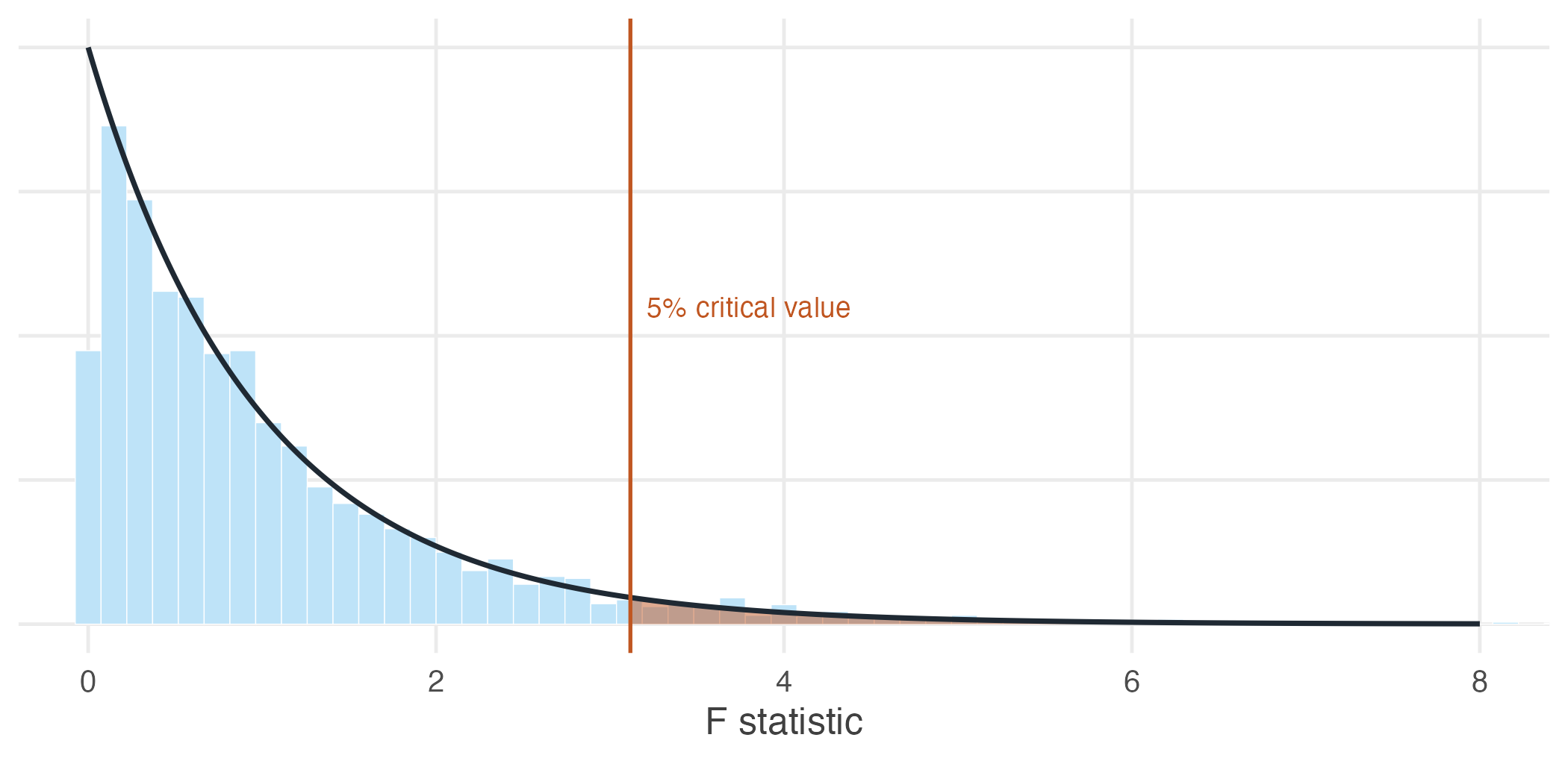
Figure 8.2: Four thousand F statistics computed from data in which the two tested variables have no effect whatever, against the F distribution with 2 and 76 degrees of freedom. The shaded region beyond the 5% critical value is where the test rejects – and since the null is true here, every rejection in it is a Type I error.
The simulated quantiles match the theoretical ones closely, and the test rejects a true null about 5% of the time, which is what a 5% test is supposed to do.
Does prior record belong in the model?
Back to the question that opened this section.
restricted   <- lm(sem_gpa ~ attendance, data = students)
unrestricted <- lm(sem_gpa ~ attendance + cum_gpa + admission_score,
                   data = students)

anova(restricted, unrestricted)
#> Analysis of Variance Table
#>
#> Model 1: sem_gpa ~ attendance
#> Model 2: sem_gpa ~ attendance + cum_gpa + admission_score
#> Res.Df RSS Df Sum of Sq F Pr(>F)
#> 1 678 1581
#> 2 676 1054 2 527 169 <0.0000000000000002 ***
#> ---
#> Signif. codes: 0 '***' 0.001 '**' 0.01 '*' 0.05 '.' 0.1 ' ' 1By hand, from the two sums of squared residuals:
ssr_r  <- sum(residuals(restricted)^2)
ssr_ur <- sum(residuals(unrestricted)^2)
q <- 2; n <- nrow(students); k <- 3

f_stat <- ((ssr_r - ssr_ur) / q) / (ssr_ur / (n - k - 1))

round(c(ssr_restricted = ssr_r, ssr_unrestricted = ssr_ur,
        F = f_stat, critical_5pct = qf(0.95, q, n - k - 1),
        p_value = 1 - pf(f_stat, q, n - k - 1)), 4)
#> ssr_restricted ssr_unrestricted F critical_5pct
#> 1580.858 1054.233 168.842 3.009
#> p_value
#> 0.000\(F = 168.8\) against a critical value of 3.01. Prior GPA and admission score belong in the model, jointly and emphatically.
The F statistic R prints by itself
Every regression summary ends with a line reporting an \(F\) statistic. It is this same test applied to one particular null: that all the slope coefficients are zero at once.
#> value numdf dendf
#> 266.8   3.0 676.0
The restricted model in that comparison has no explanatory variables at all — it predicts \(\bar{y}\) for everyone — so \(R^2_r = 0\) and the formula reduces to
\[F = \frac{R^2/k}{(1-R^2)/(n-k-1)}\]
This is the least interesting test in the output.
It asks whether the model explains anything whatever. With reasonable data and sensible variables it is almost always rejected, and rejecting it establishes very little. It is worth noticing chiefly when it fails to reject.
A joint test that does not reject
Not every set of variables earns its place. The data also record which year of the programme each student is in.
with_years <- lm(sem_gpa ~ attendance + cum_gpa + admission_score + year1 + year2,
                 data = students)

anova(unrestricted, with_years)
#> Analysis of Variance Table
#>
#> Model 1: sem_gpa ~ attendance + cum_gpa + admission_score
#> Model 2: sem_gpa ~ attendance + cum_gpa + admission_score + year1 + year2
#> Res.Df RSS Df Sum of Sq F Pr(>F)
#> 1 676 1054
#> 2 674 1051 2 3.2 1.02 0.36\(F = 1.02\) with a \(p\)-value of 0.36. Once attendance and prior record are accounted for, year of study adds nothing detectable.
Failing to reject is not proof that year of study is irrelevant, for the reason given in Section 4.9: a test that does not reject may simply lack the power to detect a small effect.
The honest statement is that these data provide no evidence that year of study matters once the other variables are held fixed.