7.2 What the fitted line guarantees
Having minimised the squares, what do we get for free?
Three algebraic facts follow directly from the two equations we just solved. They hold for every OLS regression, in every dataset, whether or not the model is any good.
- The residuals sum to zero: \(\sum \hat{u}_i = 0\). This is the first normal equation, restated.
- The residuals are uncorrelated with \(x\): \(\sum x_i \hat{u}_i = 0\). Whatever pattern is left over, it is not linearly related to \(x\) — OLS has already extracted all of that.
- The line passes through the means: \(\bar{y} = \hat{\beta}_0 + \hat{\beta}_1\bar{x}\). The point \((\bar{x}, \bar{y})\) always lies on the fitted line.
u_hat <- residuals(fit)

c(sum_residuals   = sum(u_hat),
  sum_x_times_u   = sum(x * u_hat),
  predicted_at_xbar = coef(fit)[1] + coef(fit)[2] * mean(x),
  mean_of_y         = mean(y))
#> sum_residuals sum_x_times_u
#> -0.0000000000000111 0.0000000000009965
#> predicted_at_xbar.(Intercept) mean_of_y
#> 6.5025367647058836 6.5025367647058827The first two are zero up to floating-point error, and the last two agree.
These are algebraic properties, not evidence. They hold by construction, so finding them in your output tells you the arithmetic worked and nothing more.
In particular, \(\sum x_i \hat{u}_i = 0\) is true whether or not \(E(u \mid x) = 0\). The first is forced by the estimator; the second is an assumption about the world that no computation can verify.
How much of the variation has the line accounted for?
The fitted line runs through the data, but how much of what we see does it actually capture? Answering that begins with a single observation, and requires no algebra at all.
Take one student — number 554 in the data, who attended 9 classes and finished with a semester GPA of 0.8. The class average is 6.50, so this student sits a long way below it.
That gap can be split in two.
Part of it is anticipated by the line. This student attended only 9 classes, and the line predicts a GPA of 3.26 for such a student — already well below average. The rest is not anticipated at all: the line said 3.26 and the student scored 0.8.
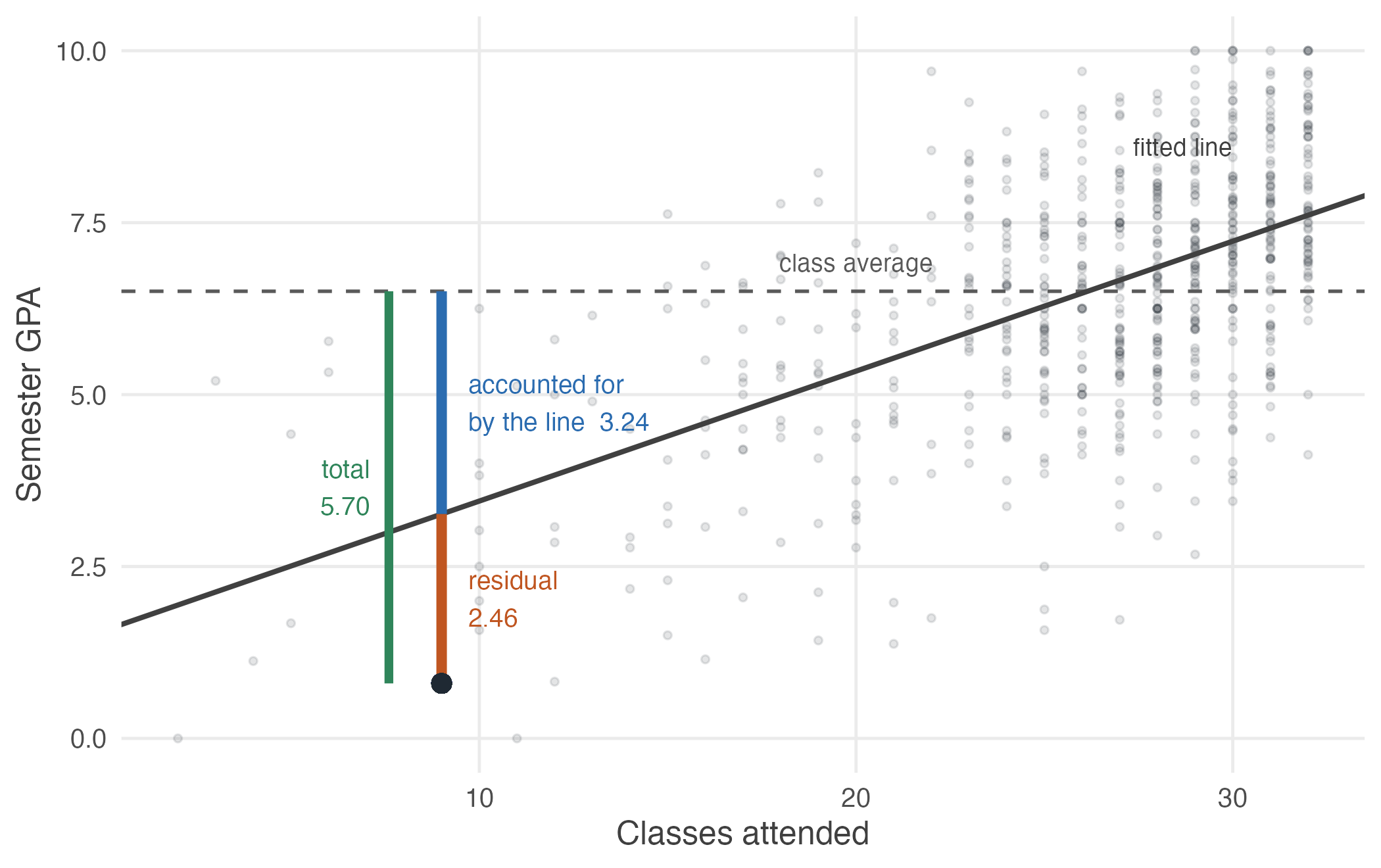
Figure 7.2: One student’s distance from the class average, split in two. The green segment is the total gap between this student and the mean. The blue segment is the part the fitted line accounts for – this student attended few classes, and the line predicts a low grade. The orange segment is what the line does not account for. The two pieces add exactly to the whole.
Read the three segments and the arithmetic is immediate:
\[\underbrace{(y_i - \bar{y})}_{\text{total}} = \underbrace{(\hat{y}_i - \bar{y})}_{\text{accounted for}} + \underbrace{(y_i - \hat{y}_i)}_{\text{residual}}\]
For this student, \(-5.70 = -3.24 + (-2.46)\).
Every observation’s distance from the mean splits into two parts: the part the fitted line accounts for, and the part it does not.
\[\text{total} = \text{accounted for by the line} + \text{residual}\]
That identity is not an approximation. Adding \(\hat{y}_i\) and subtracting it again changes nothing, so it holds exactly, for every observation, in every dataset.
From one observation to all of them
Now do the same for all 680 students. Square each distance so that departures above and below the mean do not cancel — the same reason we squared residuals in Section 6.7 — and add:
\[\sum(y_i - \bar{y})^2 = \sum(\hat{y}_i - \bar{y})^2 + \sum(y_i - \hat{y}_i)^2\]
The cross-term that ought to appear when squaring a sum vanishes exactly, and it does so because of property 2 above: the residuals are uncorrelated with \(x\), and therefore with \(\hat{y}\), which is a linear function of \(x\). That algebraic identity is what makes this decomposition work at all.
Only now are the names worth having.
| Quantity | Name | What it measures |
|---|---|---|
| \(\sum(y_i - \bar{y})^2\) | SST, total sum of squares | All the variation in \(y\) |
| \(\sum(\hat{y}_i - \bar{y})^2\) | SSE, explained sum of squares | The part the line accounts for |
| \(\sum \hat{u}_i^2\) | SSR, residual sum of squares | The part it does not |
\[\text{SST} = \text{SSE} + \text{SSR}\]
“Explained” is conventional and overstates the case. The line has accounted for that variation in an arithmetic sense; whether it has explained anything depends on whether the model is appropriate and the relationship causal.
Nothing in SSE establishes that attendance produces grades. A regression of grades on shoe size would produce a perfectly respectable SSE in a sample of children, where both rise with age.
The coefficient of determination
Dividing through by SST turns the decomposition into shares.
\[R^2 = \frac{\text{SSE}}{\text{SST}} = 1 - \frac{\text{SSR}}{\text{SST}}\]
\(R^2\) is the proportion of the variation in \(y\) accounted for by the regression. It lies between 0 and 1, and in a simple regression it is exactly the square of the correlation between \(x\) and \(y\).
sst <- sum((y - mean(y))^2)
sse <- sum((fitted(fit) - mean(y))^2)
ssr <- sum(u_hat^2)

round(c(SST = sst, SSE = sse, SSR = ssr, SSE_plus_SSR = sse + ssr), 2)
#> SST SSE SSR SSE_plus_SSR
#> 2302.2 721.4 1580.9 2302.2c(r_squared = sse / sst,
one_minus = 1 - ssr / sst,
from_summary = summary(fit)$r.squared,
cor_squared = cor(x, y)^2)#> r_squared one_minus from_summary cor_squared
#> 0.3133 0.3133 0.3133 0.3133SSE and SSR add to SST exactly, and all four routes to \(R^2\) agree.
So attendance accounts for about 31% of the variation in semester GPA. The other 69% is everything else — ability, effort, subject, luck — which is to say, the error term of Section 6.4 measured as a share.
A low \(R^2\) does not mean a regression is useless, and a high one does not mean it is right.
\(R^2\) measures how tightly the points cluster around the line. It says nothing about whether \(\beta_1\) is estimated accurately, and nothing whatever about whether the relationship is causal.
In economics, \(R^2\) values of 0.1 or 0.2 are common and unremarkable. Human behaviour is not tidy, and a model that accounted for most of the variation in something like earnings would be more suspicious than impressive.