9.6 Squares, and choosing a form

Logs impose one particular curve. What if the relationship rises and then flattens?

Logarithms bend a straight line, but they bend it in only one way: the effect of \(x\) shrinks proportionally as \(x\) grows, and it never changes sign.

Many economic relationships have a different shape. Output rises with capital, but each additional machine adds less than the last. Earnings rise with experience, then flatten and eventually fall. These are relationships with diminishing returns, and a second kind of transformation captures them.

Adding a squared term

Include the variable twice, once as itself and once squared:

\[y = \beta_0 + \beta_1 x + \beta_2 x^2 + u\]

This is still a linear regression. Nothing about the estimation changes, because linearity was always a requirement on the parameters, not on the variables. As far as OLS is concerned, \(x^2\) is just another column.

What changes is that the effect of \(x\) is no longer a single number.

Differentiating with respect to \(x\),

\[\frac{\partial y}{\partial x} = \beta_1 + 2\beta_2 x\]

The marginal effect depends on where you are. If \(\beta_1 > 0\) and \(\beta_2 < 0\), the effect is positive but shrinking — diminishing returns.

Setting the derivative to zero gives the point at which the relationship turns:

\[x^{*} = -\frac{\beta_1}{2\beta_2}\]

\(\beta_1\) on its own is now meaningless.

It is the marginal effect at \(x = 0\), which is often a value no observation comes close to. Reporting it as “the effect of \(x\)” is one of the most common errors in applied work.

With a squared term in the model, the effect must be evaluated at particular values of \(x\), and those values should be stated.

Diminishing returns to capital

The india-production.csv data record output, labour and capital for the Indian economy over forty years. Economic theory has a firm prediction here: output per worker should rise with capital per worker, but at a decreasing rate.

prod <- read.csv("data/india-production.csv")

linear <- lm(ybyl ~ kbyl, data = prod)
quad   <- lm(ybyl ~ kbyl + I(kbyl^2), data = prod)

round(coef(summary(quad)), 6)

#>              Estimate Std. Error t value Pr(>|t|)
#> (Intercept)  0.130507   0.307408  0.4245 0.673630
#> kbyl         0.343602   0.015779 21.7757 0.000000
#> I(kbyl^2)   -0.000587   0.000159 -3.6994 0.000699

The squared term is negative and significant, which is diminishing returns appearing in the data rather than only in the theory.

Note the syntax. I(kbyl^2) wraps the expression in I() so that R treats ^ as arithmetic rather than as formula notation.

b <- coef(quad)

marginal <- function(k) b["kbyl"] + 2 * b["I(kbyl^2)"] * k

round(c(at_k_20 = marginal(20), at_k_50 = marginal(50), at_k_80 = marginal(80),
        turning_point = unname(-b["kbyl"] / (2 * b["I(kbyl^2)"])),
        max_observed  = max(prod$kbyl)), 4)

#>  at_k_20.kbyl  at_k_50.kbyl  at_k_80.kbyl turning_point  max_observed 
#>        0.3201        0.2849        0.2497      292.8300       88.1205

At a capital–labour ratio of 20, one more unit of capital per worker raises output per worker by 0.32. At 80, the same addition is worth 0.25 — about a quarter less. That decline is the diminishing return.

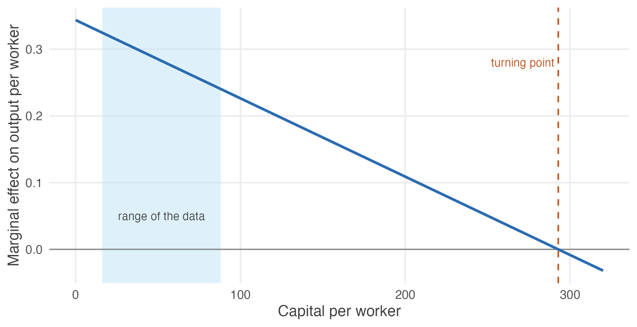
Figure 9.2: The marginal effect of capital per worker, from the fitted quadratic. It slopes downward – each additional unit of capital is worth less than the last, which is what diminishing returns means. The shaded band is the range actually observed in the data. The marginal effect stays comfortably positive throughout it, reaching zero only at 292.8, more than three times the largest value ever recorded.

Always locate the turning point before believing it.

Here it sits at 292.8, while the largest capital–labour ratio ever observed is 88.1. The model therefore says returns are positive and diminishing across the entire range of the data, and never predicts that more capital reduces output.

Had the turning point fallen inside the observed range, the model would be claiming a genuine reversal, and that claim would need defending. A quadratic is a flexible curve fitted to data, not a law. It will happily place a peak wherever the arithmetic puts one, including in places no economist would.

A squared term and a logarithm both produce a curve that flattens, and they are often near-substitutes in practice.

The difference is what happens at the ends. A log rises without limit and never turns down. A quadratic must turn, since a parabola has a peak.

If theory says the effect flattens but never reverses — as with output and capital — a log is the safer choice. If theory says the relationship genuinely peaks, as with age and earnings, the quadratic says so and the log cannot.

Choosing a form

Four considerations, in order of importance.

What is the natural way to talk about the variable? Wages, prices and GDP are discussed in percentages, so logs. Test scores, class attendance and family size are discussed in units, so levels.

Does the relationship look multiplicative? If a proportional change in \(x\) plausibly produces a proportional change in \(y\) — as with weight and fuel use — logs will fit better and mean more.

Does the scatter suggest it? Skewed variables often straighten out in logs, and heteroskedasticity often shrinks at the same time.

Does the effect plausibly change as \(x\) grows? If theory predicts diminishing returns or a peak, a squared term states that directly and can be tested with the \(t\) statistic on \(\beta_2\).

There is no universally correct transformation. There is only the one that best matches the economic question being asked.

What should not drive the choice is which version gives the larger \(R^2\) or the smaller \(p\)-value. Trying transformations until something is significant produces findings that will not replicate — and Section 9.9 explains why \(R^2\) is particularly unsuited to settling the question.

The problem of zeros

Logarithms are undefined at zero and for negative numbers.

Earnings data routinely contain zeros — people who did not work. Land holdings contain zeros for the landless. Firm exports contain zeros for firms that sell only at home.

Taking logs of such a variable does not fail loudly. R returns -Inf, lm() drops those rows, and the regression proceeds on a smaller sample without comment.

That silence is the danger. The observations lost are almost never a random subset — the landless differ from the landed in every way that matters — so the surviving regression answers a question about a different population from the one that was asked.

sum(wages$annual_earnings <= 0)

#> [1] 0

There are none here, which is a property of this simulated dataset rather than of earnings data in general.

The usual patch

The common response is to add one before taking the logarithm:

\[\ln(x + 1)\]

This is defined at zero, since \(\ln(1) = 0\), and for values much larger than 1 it is barely distinguishable from \(\ln x\). Every observation is kept and the coefficient still reads roughly as a percentage.

x <- c(0, 1, 10, 100, 10000)

print(rbind(x       = x,
            log_x   = suppressWarnings(log(x)),
            log_x_1 = log1p(x)), digits = 6)

#>         [,1]     [,2]     [,3]      [,4]        [,5]
#> x          0 1.000000 10.00000 100.00000 10000.00000
#> log_x   -Inf 0.000000  2.30259   4.60517     9.21034
#> log_x_1    0 0.693147  2.39790   4.61512     9.21044

At \(x = 10{,}000\) the two agree until the fourth decimal place. At \(x = 0\) one is undefined and the other is zero.

Notice where they disagree. At \(x = 1\) the gap is 0.69, and at \(x = 10\) it is still 0.095. The transformation leaves large values essentially untouched and changes the small ones — which are exactly the observations it was introduced to rescue. R provides log1p() for this, which is more accurate than log(x + 1) when \(x\) is very small.

The choice of 1 is arbitrary, and it is not innocent.

Nothing privileges 1 over 0.01 or 1,000. The number is not a property of the data; it is a decision by the analyst, and the estimated coefficient depends on which decision was taken. Adding a different constant gives a different answer, and the sensible-looking default is sensible only because earnings happen to be measured in units where 1 is small.

This also means the coefficient is no longer quite an elasticity. Near zero, \(\ln(x+1)\) and \(\ln x\) behave completely differently, and it is precisely the zero observations that motivated the transformation in the first place.

Use \(\ln(x+1)\) if you must, report that you did, and check whether the results survive a different constant. Better methods exist that handle zeros without inventing a constant at all, and this book returns to them once the necessary machinery is in place.

The deeper point is that a zero is often not a small number. It is a different kind of outcome.

A household earning nothing has not merely earned a very small amount; someone in it decided not to work, or could not find work. A firm exporting nothing faces a different decision from one exporting a little.

Transformations try to squeeze both decisions onto one scale. Sometimes that is acceptable. Often the zeros are the interesting part of the problem, and the honest response is to model them rather than to transform them away.