6.6 From the population to a sample

The PRF describes a population we cannot see. What do we actually have?

The population regression function is a population object. So are \(\beta_0\) and \(\beta_1\): they are fixed, unknown numbers describing every member of the population, exactly like \(\mu\) in Unit 2.

We never observe the population. What we observe is a sample of \(y\) values with their corresponding \(x\) values.

We therefore estimate. From the sample we compute \(\hat{\beta}_0\) and \(\hat{\beta}_1\), and these define the sample regression function:

\[\hat{y}_i = \hat{\beta}_0 + \hat{\beta}_1 x_i\]

where \(\hat{y}\) estimates \(E(Y \mid X = x)\), and \(\hat{\beta}_0\) and \(\hat{\beta}_1\) estimate \(\beta_0\) and \(\beta_1\).

Two sections, two lines

Suppose two sections of thirty students each are surveyed, and a line is fitted to each. Which one is the population regression function?

set.seed(12)
shuffle <- sample(nrow(students))

section_a <- students[shuffle[1:30], ]
section_b <- students[shuffle[31:60], ]

round(c(section_a   = coef(lm(sem_gpa ~ attendance, section_a))[2],
        section_b   = coef(lm(sem_gpa ~ attendance, section_b))[2],
        whole_class = coef(lm(sem_gpa ~ attendance, students))[2]), 4)

#>   section_a.attendance   section_b.attendance whole_class.attendance 
#>                 0.3004                 0.1621                 0.1890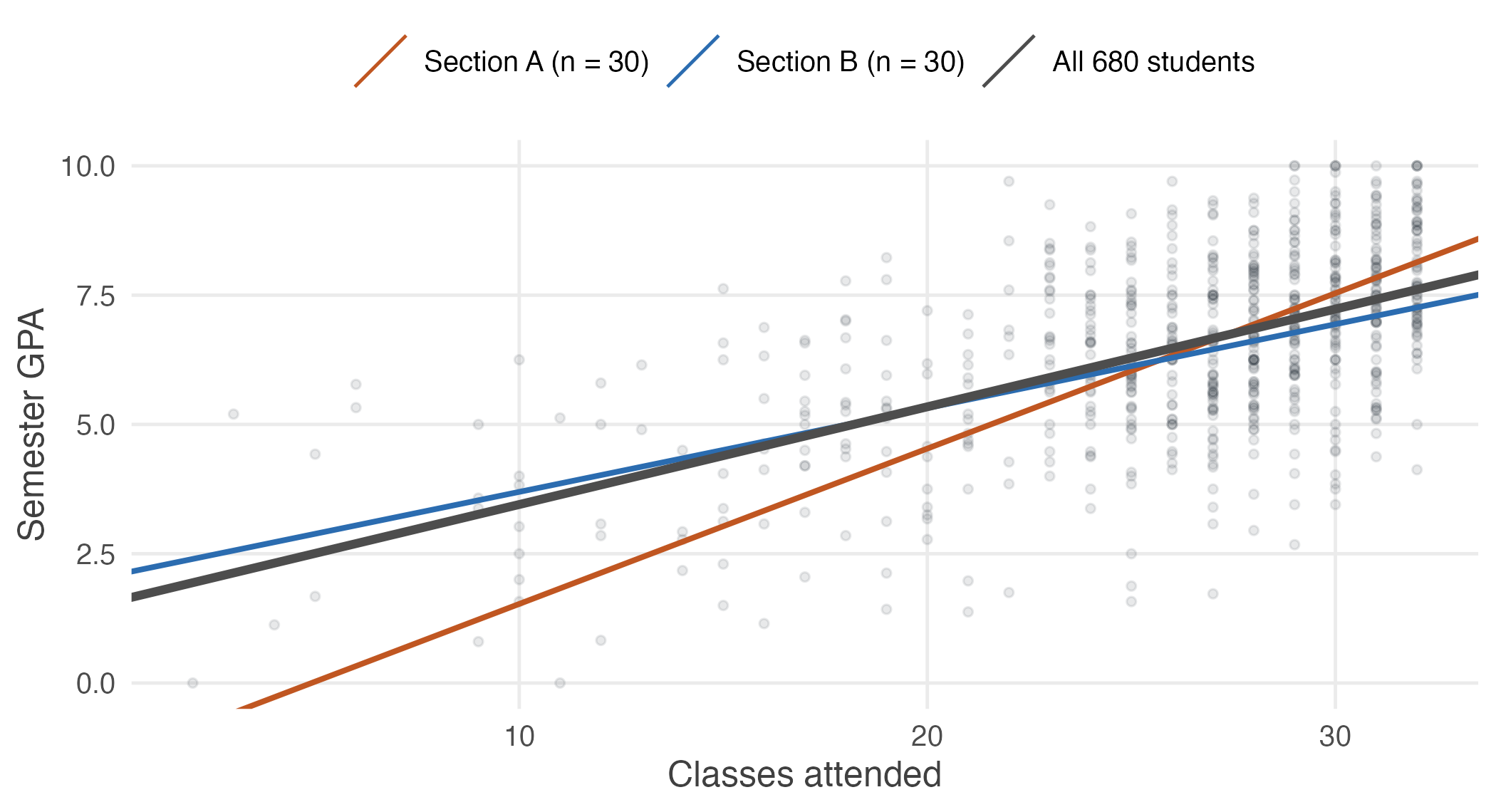

Two sections of thirty students, each with its own fitted line, against the line fitted to all 680. Neither section's line is the population regression function, and from a single section there would be no way to tell how far off it was.

Figure 6.2: Two sections of thirty students, each with its own fitted line, against the line fitted to all 680. Neither section’s line is the population regression function, and from a single section there would be no way to tell how far off it was.

There is no way to tell. Section A’s slope is 0.300 and Section B’s is 0.162 — one is nearly twice the other, and both come from the same class. A third section would give a third answer.

This is the situation of Unit 2 in a new costume. The estimate varies from sample to sample, and our task is to understand how much and why. Notice too that the two sections of thirty scatter far more widely around the full-sample line than two halves of a large sample would — which is the \(\sqrt{n}\) lesson of Unit 2 arriving in a new form.

Population (PRF)	Sample (SRF)
\(y = \beta_0 + \beta_1 x + u\)	\(y_i = \hat{\beta}_0 + \hat{\beta}_1 x_i + \hat{u}_i\)
\(y = E(Y \mid X = x) + u\)	\(y_i = \hat{y}_i + \hat{u}_i\)
\(\beta_0\) is the intercept	\(\hat{\beta}_0\) estimates \(\beta_0\)
\(\beta_1\) is the slope	\(\hat{\beta}_1\) estimates \(\beta_1\)
\(u\) is the error, and is unobservable	\(\hat{u}\) is the residual, and is computed

The distinction between \(u\) and \(\hat{u}\) is the one to hold onto. The error is the deviation from the true line, which nobody sees. The residual is the deviation from our fitted line, which we can print.

Because every sample gives a different line, \(\hat{\beta}_1\) is a random variable with a sampling distribution — and every question from Units 2 to 4 applies to it. Is it unbiased? What is its standard error? How do we test a claim about it?

Before any of that, though, we need to decide which line to fit.