9.10 Good controls and bad controls

Adding variables costs precision but not bias. So is a control ever actively harmful?

It is, and this is the most important idea in the unit.

Section 9.7 established that a variable with no effect on \(y\) is harmless. That result is narrower than it looks, because it assumed the variable’s true coefficient was zero. The dangerous cases are variables that do belong to the story — just not in the regression.

Three variables, three simulations, identical structure. In each the true effect of \(x\) on \(y\) is 1, and in each we compare the estimate with and without the control.

A variable that causes both

This is the case Unit 8 was built around. Ability raises schooling and independently raises earnings.

set.seed(19)
n <- 2000

confounder <- replicate(1500, {
  ability <- rnorm(n)
  x <- 0.7 * ability + rnorm(n)              # ability raises x
  y <- 1 * x + 1.5 * ability + rnorm(n)      # and raises y directly
  c(without_control = coef(lm(y ~ x))[2],
    with_control    = coef(lm(y ~ x + ability))[2])
})

round(rowMeans(confounder), 4)

#> without_control.x    with_control.x 
#>            1.7047            0.9998

Without the control the estimate is 1.71 against a truth of 1. With it, 1.00.

The control repaired the estimate, exactly as advertised. A variable that causes both \(x\) and \(y\) is a confounder, and controlling for it is what multiple regression is for.

A variable that x causes

Now change one thing. The added variable is not a cause of \(x\); it is a consequence of it.

Education raises occupational rank, and occupational rank raises earnings. Part of how education pays is by getting people into better jobs.

set.seed(19)

mediator <- replicate(1500, {
  educ <- rnorm(n)
  occupation <- 0.6 * educ + rnorm(n)                  # education raises rank
  earnings   <- 0.4 * educ + 1.0 * occupation + rnorm(n)
  c(without_control = coef(lm(earnings ~ educ))[2],
    with_control    = coef(lm(earnings ~ educ + occupation))[2])
})

round(rowMeans(mediator), 4)

#> without_control.educ    with_control.educ 
#>               0.9999               0.4000

The total effect of education is 1.0: a direct effect of 0.4, plus 0.6 through occupation.

Without the control we recover 1.00 — correct. With the control we get 0.40.

Controlling for occupation did not remove bias. It removed part of the effect.

Holding occupation fixed means comparing people who ended up in the same job. Among such people, education can no longer operate through the route by which most of it operates. What survives is only the direct effect.

A variable that lies on the causal path from \(x\) to \(y\) is a mediator, and controlling for it answers a narrower question than the one asked — often without the researcher noticing that the question changed.

A variable that both x and the error cause

The third case is the least intuitive and the most damaging.

Suppose \(x\) has a genuine effect on \(y\) and there is no confounding whatever, so a simple regression would have been correct. Now control for a variable that is caused by both \(x\) and the unobserved part of \(y\).

set.seed(19)

collider <- replicate(1500, {
  x <- rnorm(n)
  u <- rnorm(n)                                  # unobserved, affects y
  y <- 1 * x + u                                 # no confounding: x and u independent
  selected <- 0.8 * x + 0.8 * u + rnorm(n)       # caused by both
  c(without_control = coef(lm(y ~ x))[2],
    with_control    = coef(lm(y ~ x + selected))[2])
})

round(rowMeans(collider), 4)

#> without_control.x    with_control.x 
#>              1.00              0.61

Without the control the estimate is 1.00, and correctly so — there was nothing to correct.

Adding the control breaks it, giving 0.61.

Here the control created bias where none existed.

A variable caused by both \(x\) and the error term is a collider. Conditioning on it induces a relationship between \(x\) and \(u\) that was not there before, which is precisely the failure of CLRM4 that Unit 8 warned about — manufactured by the researcher.

The mechanism is easier to see in a concrete case.

Suppose a firm hires workers who are either well-qualified or visibly talented, and that qualifications and talent are unrelated in the population at large. Among the people it hires, the two will be negatively related: someone hired despite weak qualifications must have been unusually talented, and the reverse.

Restricting attention to those hired — or controlling for being hired — manufactures a correlation between two things that were independent.

This is why controlling for variables measured after the treatment, or for anything determining who appears in the sample, is dangerous in a way that has nothing to do with sample size.

What this means in practice

The three simulations are identical in form. Each adds one control to a regression, and the results are opposite.

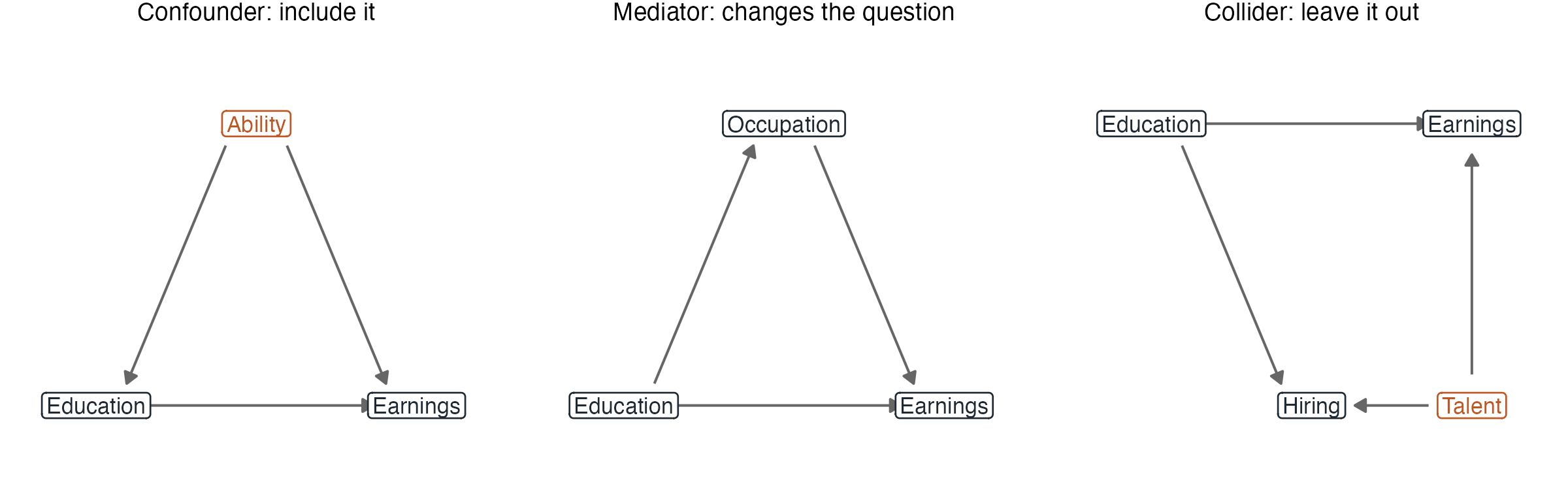
Figure 9.3: The three cases as pictures. Arrows run from cause to effect, and variables in orange are unobserved. The first two are the same triangle with the arrows reversed – ability causes education, whereas education causes occupation – and that reversal is the whole difference between a control that repairs an estimate and one that destroys it. In the third, two arrows run into hiring, which is what makes it a collider.

Table 9.2: The same operation, three times, with three different consequences. The true effect is 1 in every case.

The control is	Without it	With it	Verdict
A cause of \(x\) and \(y\) (confounder)	1.71	1.00	Include it
Caused by \(x\) (mediator)	1.00	0.40	Changes the question
Caused by \(x\) and by \(u\) (collider)	1.00	0.61	Leave it out

No property of the data distinguishes these three cases.

All three controls are correlated with \(x\) and with \(y\). All three change the coefficient. All three are statistically significant. Every diagnostic in this book passes in all three regressions.

What separates them is the direction of causation between the variables — which is knowledge about the world, not a fact the sample contains.

The common practice of adding every available variable and reporting whichever specification looks best is not caution. It is an invitation to all three problems at once, and it is undetectable in the results.

This is the honest answer to “which variables should I control for?” It requires an argument about what causes what, made before the regression is run and defended in the text.

The question cannot be settled by looking at output.