2.5 Why do larger samples fluctuate less?

Unbiasedness cannot be the whole story. What does a larger sample actually buy?

Unbiasedness alone is worth remarkably little. Consider the rule “take the first observation and ignore the rest.” It is perfectly unbiased — \(E(X_1) = \mu\) — and nobody would use it, because it never improves. Collect a million households and it still reports one household’s income.

So the second property has to concern spread. Run the deck experiment across a range of sample sizes.

set.seed(7)

sizes <- c(5, 10, 20, 40, 80)
results <- t(sapply(sizes, function(n) {
  m <- replicate(2000, mean(sample(deck, size = n, replace = TRUE)))
  c(n = n, mean = mean(m), sd = sd(m), theoretical_sd = sd(deck) / sqrt(n))
}))

round(results, 3)

#>       n  mean    sd theoretical_sd
#> [1,]  5 6.932 1.688          1.690
#> [2,] 10 7.022 1.165          1.195
#> [3,] 20 7.009 0.845          0.845
#> [4,] 40 7.019 0.597          0.597
#> [5,] 80 6.996 0.415          0.422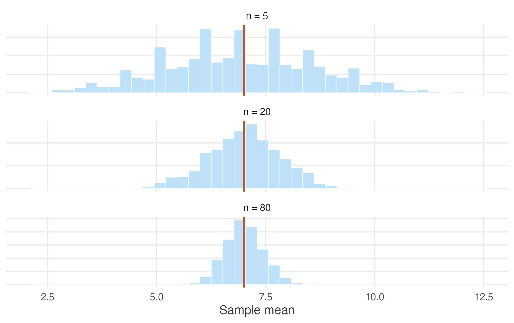

Figure 2.3: Sampling distributions of the mean for growing sample sizes. The centre never moves. The spread collapses.

The second column confirms the previous section: every sample size is centred on 7, and even samples of five are centred correctly. Centring does not improve with \(n\), because it was never wrong.

The third column is what changes. At \(n = 5\) the sample means have a standard deviation of about 1.69; at \(n = 80\) it is about 0.42. Compare it against the fourth column: the observed spread matches \(\sigma/\sqrt{n}\) almost exactly at every sample size.

\[ \begin{aligned} \mathrm{Var}(\bar{X}) &= \mathrm{Var}\!\left(\frac{1}{n}(X_1 + \cdots + X_n)\right) \\[4pt] &= \frac{1}{n^2}\,\mathrm{Var}(X_1 + \cdots + X_n) \\[4pt] &= \frac{1}{n^2}\underbrace{(\sigma^2 + \sigma^2 + \cdots + \sigma^2)}_{n \text{ times}} \\[4pt] &= \frac{n\sigma^2}{n^2} \;=\; \frac{\sigma^2}{n} \end{aligned} \]

The second line uses \(\mathrm{Var}(aX) = a^2\mathrm{Var}(X)\). The third line is the one that matters: the variance of a sum equals the sum of the variances only when the observations are independent. This is the single point in the entire argument at which independence is required.

Survey C is now explained. Its households were drawn from the right population, so it stayed centred — but they were not independent, the third line above did not hold, and the true spread was more than three times what \(\sigma/\sqrt{n}\) claimed. A researcher who applied the formula anyway would have reported a precision the data did not contain.

The square root of this variance is used so constantly that it has its own name.

The standard error of the sample mean is the standard deviation of its sampling distribution:

\[\mathrm{se}(\bar{X}) = \sqrt{\mathrm{Var}(\bar{X})} = \frac{\sigma}{\sqrt{n}}\]

It measures how much the sample mean moves from sample to sample. A small standard error means that whatever answer we happened to get, a different sample would have given something similar.

The word error is unfortunate, and worth guarding against. It does not measure a mistake, and it is not the distance between your estimate and the truth — that distance is unknowable. Like unbiasedness, it is a property of the procedure.