1.10 Practice problems
These are for learning. Work each one before opening the solution; the answer is worth very little if you have not first tried to produce it yourself.
The question bank that follows is for testing yourself and has no answers at all.
Concept checks
Short questions. A sentence or two is enough.
1.1 Why does repeating the same survey produce a different average each time?
Because a different set of people is surveyed each time. Every average is computed from whoever happened to be selected, and selection involves chance. The population has not changed and no arithmetic error has occurred — only the membership of the sample.
1.2 A die with a three painted on all six faces is rolled ten thousand times. What is the distribution of the outcome? Why is this example in the chapter at all?
There is no distribution to speak of: every outcome is three, and the standard deviation is zero. The example is there to show that statistics requires variation. Where outcomes never differ, there is nothing to describe, nothing to be uncertain about, and no inference to perform.
1.3 Distinguish between \(\bar{X}\) and \(\bar{x}\).
\(\bar{X}\) is the sample mean regarded as a random variable, before the sample is drawn: it has a distribution, a centre and a spread. \(\bar{x}\) is the single number obtained once a particular sample has been collected — one realisation of \(\bar{X}\).
1.4 A survey of 400 households gives a mean monthly income of ₹18,000. Is ₹18,000 a parameter or a statistic? What is the parameter here?
₹18,000 is a statistic: it was computed from a sample and would change with a different sample. The parameter is the mean monthly income of the whole population, \(\mu\), which is fixed but unknown.
Explain
One paragraph each. These reward clarity rather than calculation.
1.5 Explain to a friend who has never studied statistics why the Law of Large Numbers does not mean that a large sample is guaranteed to give the right answer.
The law says that as the sample grows, the sample mean becomes increasingly likely to lie close to the population mean — not that it will equal it. Any particular large sample may still be unlucky. What changes with sample size is the probability of being far off, which shrinks; the possibility never disappears. A large sample makes a badly wrong answer improbable, not impossible.
1.6 A friend argues that because a coin has landed heads six times running, tails is now more likely. Using the Law of Large Numbers, explain why this is wrong.
The coin has no memory, and the law promises nothing of the kind. What converges is the proportion of heads, and it converges by dilution rather than by correction. The six extra heads are never cancelled out; they simply become a smaller and smaller share of a growing total. The absolute surplus of heads typically grows with the number of tosses even as the proportion approaches one half.
1.7 Two researchers study earnings in the same district. One surveys 100 households, the other 2,500. Both report a mean. Which should be trusted more, and what would you need to know before answering?
Other things equal, the larger survey has the smaller standard deviation of the sample mean — by a factor of five, since \(\sqrt{2500/100} = 5\). But this holds only if both samples were drawn from the population of interest and drawn at random. A carefully designed survey of 100 households is worth more than a badly drawn survey of 2,500. Sample size governs precision; sampling design governs whether precision is about the right quantity at all.
Numerical problems
Work each of these with a pen first. Each ends by asking you to check your answer by simulation — the point being that theory and simulation should agree, and that when they do not, one of them is wrong.
1.8 The earnings data used throughout this chapter has a population mean of about ₹54,200 and a population standard deviation of about ₹100,100.
Suppose a survey team draws random samples of (a) 50, (b) 100, (c) 200 and (d) 1,000 workers.
- Find the expected value of the sample mean in each case.
- Find the standard deviation of the sample mean in each case.
- What happens to that standard deviation as the sample size increases, and why?
- Verify your answers by simulation.
The expected value of the sample mean equals the population mean whatever the sample size, so \(E(\bar{X}) = ₹54{,}200\) in all four cases. Sample size affects precision, not location.
The standard deviation of the sample mean is \(\sigma/\sqrt{n} = 100{,}100/\sqrt{n}\):
sigma <- 100100
n     <- c(50, 100, 200, 1000)

round(data.frame(n, expected = 54200, se = sigma / sqrt(n)))
#> n expected se
#> 1 50 54200 14156
#> 2 100 54200 10010
#> 3 200 54200 7078
#> 4 1000 54200 3165It falls in proportion to \(1/\sqrt{n}\). Each additional worker contributes information, so the average over many of them is pulled more tightly around the population value. Note that raising the sample from 50 to 1,000 — twenty times the data — reduces it only by a factor of \(\sqrt{20} \approx 4.5\).
Because we hold the whole population, the answer can be checked directly:
set.seed(4)
earn <- read.csv("data/wages-india-synthetic.csv")$annual_earnings

sim <- sapply(n, function(k)
  sd(replicate(2000, mean(sample(earn, k, replace = TRUE)))))

round(data.frame(n, theoretical = sd(earn) / sqrt(n), simulated = sim))
#> n theoretical simulated
#> 1 50 14162 14219
#> 2 100 10014 9740
#> 3 200 7081 7204
#> 4 1000 3167 3120The two columns agree closely. The small discrepancies are themselves sampling variation: each simulated standard deviation is estimated from 2,000 samples rather than infinitely many.
1.9 An auto-rickshaw driver’s daily earnings vary from day to day, with a mean of ₹800 and a standard deviation of ₹200. In a particular month the driver works 30 days.
- What are the mean and standard deviation of total earnings for the month?
- Approximate the probability that the month’s total exceeds ₹25,000.
- Approximate the probability that it falls below ₹22,000.
- Approximate the probability that it lies between ₹22,000 and ₹25,000.
- What assumption does this calculation require, and is it plausible here?
- Check your answers by simulating 10,000 months.
The monthly total is a sum of 30 daily earnings. Its mean is \(30 \times 800 = ₹24{,}000\), and because variances add for independent quantities, its standard deviation is \(200\sqrt{30} = ₹1{,}095\).
By the Central Limit Theorem the total is approximately normal, so:
mu_day <- 800; sd_day <- 200; days <- 30

mu_tot <- mu_day * days
sd_tot <- sd_day * sqrt(days)

c(mean = mu_tot, sd = sd_tot,
  above_25000 = pnorm(25000, mu_tot, sd_tot, lower.tail = FALSE),
  below_22000 = pnorm(22000, mu_tot, sd_tot),
  between     = pnorm(25000, mu_tot, sd_tot) - pnorm(22000, mu_tot, sd_tot))
#> mean sd above_25000 below_22000 between
#> 24000.00000 1095.44512 0.18066 0.03394 0.78540So roughly an 18% chance of clearing ₹25,000, a 3% chance of falling below ₹22,000, and a 79% chance of landing between the two.
The assumption is independence. The calculation treats each day’s earnings as unrelated to every other day’s. That is questionable. A week of heavy monsoon suppresses earnings on consecutive days; a festival week raises them together. When days are positively correlated, the true standard deviation of the monthly total is larger than \(200\sqrt{30}\), and the probability of an unusually bad month is correspondingly higher than this calculation suggests.
This is worth dwelling on. The arithmetic is not wrong; the assumption is. No amount of care in the computation would reveal the problem.
Simulating under the stated assumption:
set.seed(5)
months <- replicate(10000, sum(rnorm(days, mu_day, sd_day)))

c(mean = mean(months), sd = sd(months),
  above_25000 = mean(months > 25000),
  below_22000 = mean(months < 22000),
  between     = mean(months >= 22000 & months <= 25000))
#> mean sd above_25000 below_22000 between
#> 23987.5096 1090.6065 0.1788 0.0321 0.7891The simulated proportions match the normal approximation closely — as they must, since the simulation was itself built on the assumption of independent daily earnings. Simulation confirms the arithmetic; it cannot confirm the assumption.
R exercises
1.10 Simulate the Central Limit Theorem starting from an exponential
distribution, which is strongly right-skewed. Draw 5,000 sample means for
sample sizes of 1, 5, 30 and 200 from rexp(n, rate = 1), and plot the four
distributions. At which sample size does the result begin to look normal?
set.seed(1)

sizes <- c(1, 5, 30, 200)
sim <- do.call(rbind, lapply(sizes, function(n)
  data.frame(n = factor(paste("n =", n), levels = paste("n =", sizes)),
             m = replicate(5000, mean(rexp(n, rate = 1))))))

ggplot(sim, aes(m)) +
  geom_histogram(bins = 50, fill = book_palette$fill, colour = "white",
                 linewidth = 0.1) +
  facet_wrap(~ n, scales = "free") +
  labs(x = "Sample mean", y = NULL) +
  theme_book() +
  theme(axis.text.y = element_blank())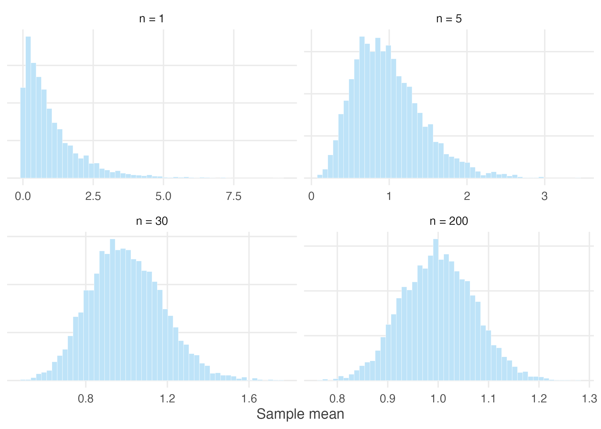
Figure 1.9: Sampling distributions of the mean from an exponential population.
At \(n = 1\) the picture is the exponential distribution itself — a sharp peak at zero with a long right tail. By \(n = 5\) it has a recognisable mound but remains clearly skewed. By \(n = 30\) it is close to symmetric, and by \(n = 200\) it is difficult to distinguish from a normal distribution by eye.
The exponential distribution has skewness 2, which is milder than the earnings data used in this chapter. That is why \(n = 30\) works reasonably well here and less well there.
1.11 Using data/cricket-toss.csv, plot each team’s toss-win percentage
against its number of matches. What shape does the scatter take, and why?
toss <- read.csv("data/cricket-toss.csv")

band <- data.frame(n = 5:2200)
band$hi <- 50 + 2 * 50 / sqrt(band$n)
band$lo <- 50 - 2 * 50 / sqrt(band$n)

ggplot(toss, aes(matches, pct_toss_won)) +
  geom_ribbon(data = band, aes(x = n, ymin = lo, ymax = hi),
              inherit.aes = FALSE, fill = book_palette$fill, alpha = 0.45) +
  geom_hline(yintercept = 50, colour = book_palette$reject, linewidth = 0.6) +
  geom_point(alpha = 0.7, size = 1.6, colour = book_palette$ink) +
  scale_x_log10(labels = scales::comma) +
  labs(x = "Matches played (log scale)", y = "Toss-win percentage") +
  theme_book()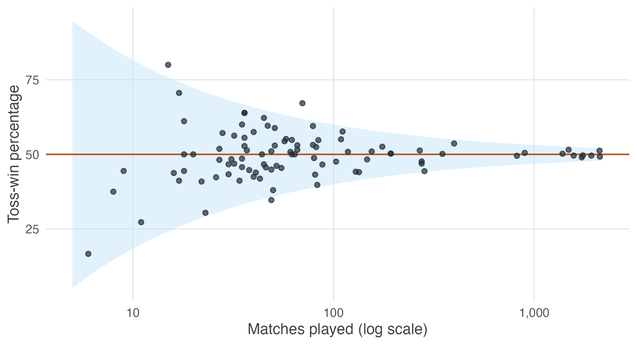
Figure 1.10: Toss-win percentage against number of matches played, with the theoretical limits of two standard deviations.
The scatter forms a funnel: wide on the left, where teams have played few matches, and narrowing towards 50% as the number of matches grows. The shaded band shows two standard deviations either side of 50, computed as \(50/\sqrt{n}\) — the same formula that governs the sample mean. Almost every team falls inside it.
This is the Law of Large Numbers made visible. The teams with extreme records are not lucky; they are simply the teams with few observations.