4.12 Practice problems
Work each one on paper first, then check yourself in R. The solutions are one click away, which makes them worth nothing unless you try first.
These are for learning, so the workings are shown in full. The question bank that follows is for testing yourself, and has no answers.
11.1 A consumer research organisation states that the mean caffeine content per 12-ounce bottle of a caffeinated soft drink is 37.7 mg. A random sample of 36 bottles has a mean of 35.28 mg. The population standard deviation is 10.8 mg. At \(\alpha = 0.01\), can you reject the organisation’s claim?
\(H_0: \mu = 37.7\) against \(H_A: \mu \neq 37.7\). Two-tailed at \(\alpha = 0.01\), so the critical value is \(Z_{0.005} = 2.58\).
\[ Z_{calc} = \frac{35.28 - 37.7}{10.8/\sqrt{36}} = \frac{-2.42}{1.8} = -1.34 \]
caffeine <- make_sample(n = 36, mean = 35.28, sd = 10.8)
z.test(caffeine, mu = 37.7, sigma.x = 10.8, conf.level = 0.99)
#>
#> One-sample z-Test
#>
#> data: caffeine
#> z = -1.3, p-value = 0.2
#> alternative hypothesis: true mean is not equal to 37.7
#> 99 percent confidence interval:
#> 30.64 39.92
#> sample estimates:
#> mean of x
#> 35.28\(|-1.34| < 2.58\) and the \(p\)-value of 0.179 is far above 0.01, so we fail to reject. If the true mean really were 37.7 mg, a sample mean this far away would turn up about 18% of the time — thoroughly unremarkable.
11.2 Historical data show household water use is normally distributed with mean 360 gallons and standard deviation 40 gallons per day. A sample of 200 households averages 374 gallons. Are these data consistent with the historical distribution at the 5% level? What is the \(p\)-value?
\[ Z_{calc} = \frac{374 - 360}{40/\sqrt{200}} = \frac{14}{2.828} = 4.95 \]
water <- make_sample(n = 200, mean = 374, sd = 40)
z.test(water, mu = 360, sigma.x = 40, conf.level = 0.95)
#>
#> One-sample z-Test
#>
#> data: water
#> z = 4.9, p-value = 0.0000007
#> alternative hypothesis: true mean is not equal to 360
#> 95 percent confidence interval:
#> 368.5 379.5
#> sample estimates:
#> mean of x
#> 374\(4.95 \gg 1.96\), and the \(p\)-value is about 0 — under one in a million. Reject \(H_0\). Water use has moved away from the historical mean.
11.3 A study claims the average monthly salary of full professors in India is ₹87,800. Students at one university sample ten salaries (in thousands):
91.0, 79.8, 102.0, 93.5, 82.0, 88.6, 90.0, 98.6, 101.0, 84.0They believe their professors earn more. Test at the 10% and 5% levels.
The word “more” makes this right-tailed: \(H_0: \mu \leq 87.8\) against \(H_A: \mu > 87.8\). Since \(\sigma\) is unknown and \(n = 10\), use a \(t\)-test with \(df = 9\).
salary <- c(91.0, 79.8, 102.0, 93.5, 82.0, 88.6, 90.0, 98.6, 101.0, 84.0)

c(mean = mean(salary), sd = sd(salary))
#> mean sd
#> 91.050 7.797#>
#> One Sample t-test
#>
#> data: salary
#> t = 1.3, df = 9, p-value = 0.1
#> alternative hypothesis: true mean is greater than 87.8
#> 95 percent confidence interval:
#> 86.53 Inf
#> sample estimates:
#> mean of x
#> 91.05\(t_{calc} = 1.318\), against critical values \(t_{0.10,\,9} = 1.383\) and \(t_{0.05,\,9} = 1.833\).
The statistic falls short of both. Fail to reject at either level — there is not enough evidence that these professors are paid above the national figure.
11.4 A Department of Transportation claims mean wait time is at most 6 minutes. A sample of 34 locations has mean 10.3 minutes, standard deviation 8.0. Test at 5% and 1%.
“At most” makes this right-tailed: \(H_0: \mu \leq 6\) against \(H_A: \mu > 6\), \(t\)-test with \(df = 33\).
#>
#>  One Sample t-test
#>
#> data:  waits
#> t = 3.1, df = 33, p-value = 0.002
#> alternative hypothesis: true mean is greater than 6
#> 95 percent confidence interval:
#>  7.978   Inf
#> sample estimates:
#> mean of x
#>      10.3
\(t_{calc} = 3.14\), well beyond \(t_{0.05,\,33} = 1.692\) and \(t_{0.01,\,33} = 2.445\). Reject at both levels — wait times are longer than claimed.
11.5 marriage-ages.csv records the ages of both partners in ten couples.
Is there evidence that one partner tends to be older? Test at the 5% level.
Hint: the two columns are not independent samples — they are ten couples. What is the one number per couple that captures the question?
The two columns are paired: each row is one couple. Treating them as two independent samples throws away that pairing and inflates the standard error. The right move is to reduce each couple to a single number — the age gap — and run a one-sample test on it against zero.
#> [1] 1 5 4 1 1 4 0 8 1 0#> mean sd n
#> 2.500 2.635 10.000#>
#> One Sample t-test
#>
#> data: gap
#> t = 3, df = 9, p-value = 0.01
#> alternative hypothesis: true mean is not equal to 0
#> 95 percent confidence interval:
#> 0.6149 4.3851
#> sample estimates:
#> mean of x
#> 2.5The mean gap is 2.5 years, \(t = 3.0\) on 9 degrees of freedom, \(p = 0.015\). Since \(0.015 < 0.05\), we reject \(H_0\): partner 1 is reliably older.
R will do the pairing for you if you ask:
#>
#>  Paired t-test
#>
#> data:  couples$partner1 and couples$partner2
#> t = 3, df = 9, p-value = 0.01
#> alternative hypothesis: true mean difference is not equal to 0
#> 95 percent confidence interval:
#>  0.6149 4.3851
#> sample estimates:
#> mean difference
#>             2.5
Identical output — paired = TRUE computes exactly the differences we formed
by hand. Compare what happens if you forget:
#> [1] 0.607The same ten couples, a \(p\)-value of 0.607 instead of 0.015, and the opposite conclusion. Pairing is not a detail.
11.6 (No computation.) A classmate reports “\(p = 0.03\), so there is a 3% chance the null hypothesis is true.” Explain what is wrong, and state what \(p = 0.03\) does mean.
The \(p\)-value is computed assuming the null is true. It cannot then also be the probability that the null is true — that would be circular. Formally, your classmate has swapped \(P(\text{data} \mid H_0)\) for \(P(H_0 \mid \text{data})\), which are different quantities entirely.
The correct reading: if \(H_0\) were true, samples at least as extreme as this one would arise 3% of the time. Since that is unusual, we treat it as evidence against \(H_0\) — but the statement is about how surprising the data are, not about how probable the hypothesis is.
Type I and Type II errors
4.15 A district administration tests whether a new teaching programme raised average test scores. State, in the language of the problem, what a Type I error and a Type II error would be, and say which you would consider more serious.
A Type I error is concluding the programme raised scores when it did not. The district would scale up an ineffective programme, spending money and teaching time that could have gone elsewhere, and would believe a problem had been solved when it had not.
A Type II error is concluding the programme did not work when it did. A genuinely effective intervention would be abandoned.
Which is worse is not a statistical question. If the programme is cheap and the alternative is doing nothing, a missed effect is the costlier error and a larger \(\alpha\) might be defensible. If scaling up is expensive and irreversible, the false alarm is worse.
The point is that \(\alpha\) encodes such a judgement whether or not anyone makes it deliberately. Choosing 0.05 out of habit is still choosing.
4.16 Explain why setting \(\alpha = 0.001\) does not make a test “more accurate”.
It makes the test less likely to raise a false alarm and more likely to miss a real effect. Lowering \(\alpha\) moves the critical value further out, which shrinks the rejection region — and the rejection region is where real effects get detected too.
Accuracy in any useful sense involves both errors. Reducing one by moving the threshold always increases the other, because the threshold is the boundary between them.
Both fall together only when the two sampling distributions move apart, which requires a larger sample, a bigger effect or less noise. That is a matter of design, not of choosing a smaller number.
4.17 A trial with \(\sigma = 4\) and \(n = 16\) tests \(H_0: \mu \leq 0\) against \(H_A: \mu > 0\) at \(\alpha = 0.05\). The true effect is \(\mu_1 = 2\).
- Compute the critical value and the standard error.
- Compute \(\beta\) and the power.
- Recompute the power at \(\alpha = 0.01\).
- What does the comparison show?
(i) One-sided at 5%: \(z_{0.05} = 1.645\). Standard error \(= 4/\sqrt{16} = 1\).
(ii) Under the alternative the statistic is centred on \(\delta = (2-0)/1 = 2\), so
\[\beta = P(Z \leq 1.645 - 2) = \Phi(-0.355) = 0.361\]
and the power is \(1 - 0.361 = 0.639\).
(iii) At \(\alpha = 0.01\) the critical value is \(z_{0.01} = 2.326\), so \(\beta = \Phi(2.326 - 2) = \Phi(0.326) = 0.628\) and the power falls to 0.372.
(iv) Tightening \(\alpha\) from 5% to 1% cut the chance of detecting a real two-point effect from 64% to 37%. The stricter test is not the better test; it has simply traded one error for the other. Nothing about the drug changed.
4.18 How large must the trial in the previous question be to detect a two-point effect with 80% power?
Power of 80% means \(\beta = 0.20\), and the critical value must sit \(z_{0.20}\) below the alternative’s centre. Since \(z_{0.20} = 0.842\), we need
\[\delta = z_{\alpha} + z_{\beta} = 1.645 + 0.842 = 2.487\]
With \(\delta = (\mu_1 - \mu_0)\sqrt{n}/\sigma\),
\[\sqrt{n} = \frac{2.487 \times 4}{2} = 4.97 \qquad\Longrightarrow\qquad n = 24.7\]
so 25 patients. Checking against the table in Section 4.9, \(n = 25\) gives power 0.804.
Note the shape of this calculation: it is done before the trial, and it requires naming the smallest effect worth detecting. That is a judgement about medicine, not statistics, and it has to be made either way.
4.19 Plot the power of the trial in question 4.17 against sample size, for true effects of one point and two points.
power_at <- function(n, effect, sigma = 4, alpha = 0.05) {
  1 - pnorm(qnorm(1 - alpha) - effect / (sigma / sqrt(n)))
}

grid <- expand.grid(n = seq(5, 250, by = 5), effect = c(1, 2))
grid$power <- power_at(grid$n, grid$effect)
grid$effect <- factor(grid$effect, labels = c("1 point", "2 points"))

ggplot(grid, aes(n, power, colour = effect)) +
  geom_hline(yintercept = 0.8, linetype = "dashed", colour = "grey45") +
  geom_line(linewidth = 0.9) +
  scale_colour_manual(values = c(book_palette$reject, book_palette$accent),
                      name = "True effect") +
  labs(x = "Sample size", y = "Power") +
  theme_book() +
  theme(legend.position = "top")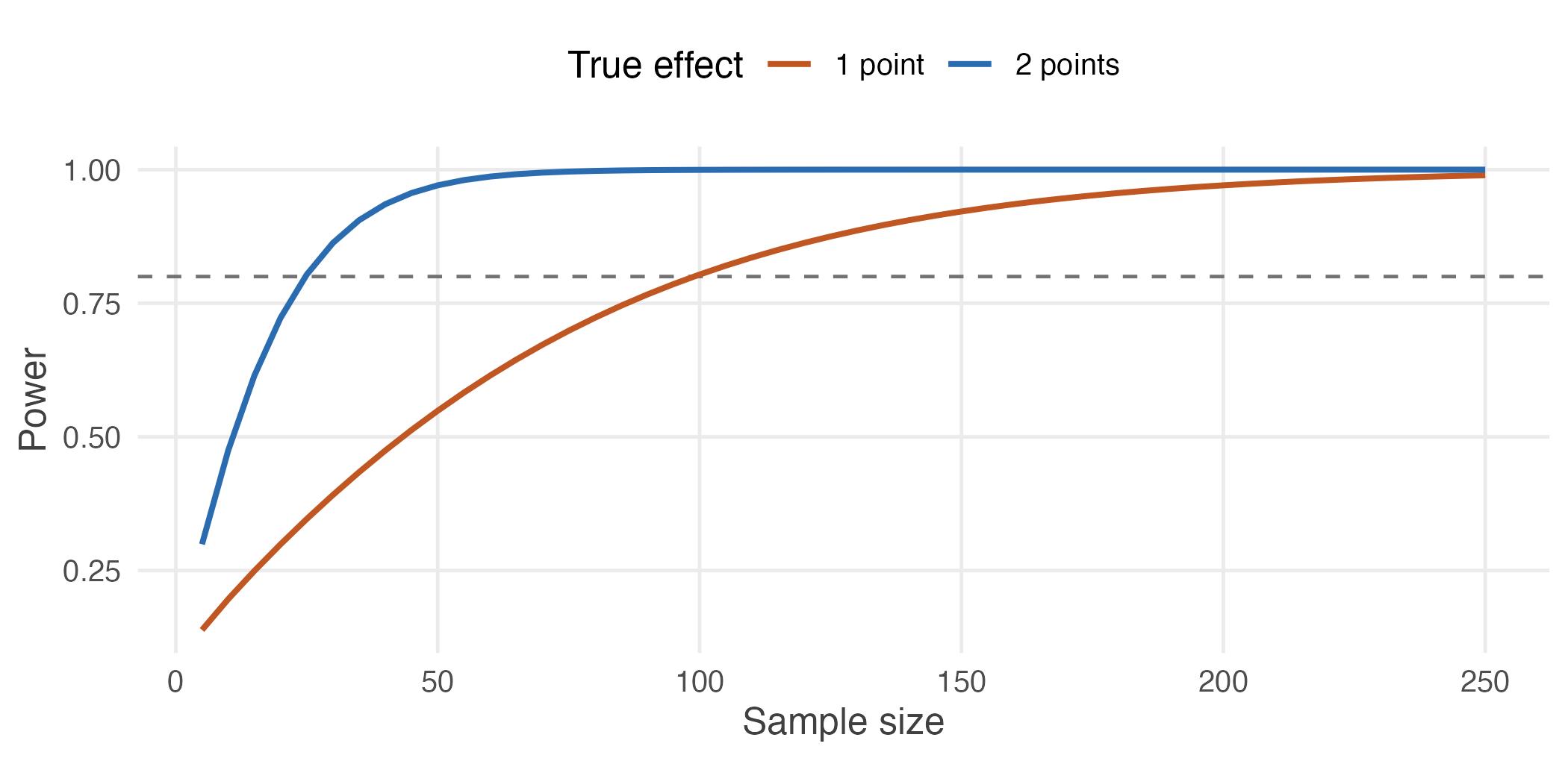
Figure 4.6: Power against sample size for two effect sizes. Small effects need far more data.
Both curves rise towards 1, and the dashed line marks the conventional 80% target. Detecting a two-point effect takes about 25 patients; detecting a one-point effect takes about 100.
Halving the effect roughly quadruples the sample needed, which is the \(\sqrt{n}\) rule appearing once more: precision improves with the square root of the sample, so detecting an effect half the size requires four times the data.